Keywords
Symptoms measurement; Two-part modeling; Community sampling; Histogram fit; Log-normal distribution; Multiplicative measurement model
Introduction
Symptoms as self-reported feelings of abnormality play a critical role in psychopathological diagnosis and assessment. Symptoms considered as overt manifestations of an underlying pathological state [1] differ from traits in that symptoms can be meaningfully reported as present or absent, whereas traits are generally considered to be ever present in some positive amount [2]. This distinction is central to an understanding of the inherent difference between human health and human ability measurement.
The Zero-problem and its ramifications
Zero as a real representation of nothing has historically fascinated mankind [3]. Measurement-wise, zero can be used to represent the total absence of a construct amount, as in absolute zero temperature, or to represent a categorical distinction of kind such as presence or absence of a disease. The problem is that zero cannot simultaneously be ascribed both a categorical and a dimensional representation within a generative experiment. Readers are encouraged to refer to [2] for a discussion of experiment as a generative process. If zero is used to designate a class, the distinction between zero and non-zero is qualitative. On the other hand, if zero is intended to distinguish absence of a construct amount from its presence, the distinction is quantitative. Of course, the digit 0 as a scale origin can always be arbitrarily assigned to an observable event, such as the freezing point of water.
Community sampling defined as the selection of experimental subjects from a community setting [4] is particularly susceptible to the zero problem. The reason is that community samples are likely to contain an admixture of asymptomatic and symptomatic individuals. Class membership as well as class proportions are usually unknown and must be estimated from sample data. Symptom presence is generally scaled on intensity, severity, frequency, or duration, with five or more integer benchmarks arranged from left to right in ascending order. Seldom is a scale benchmark provided to account for symptom absence. In the absence of an explicit zero benchmark, asymptomatic individuals are more likely to choose the leftmost benchmark indicating the least amount resulting in positively skewed response distributions.
The zero-problem has ramifications for the computation of sample mean, variance, and covariance. The inclusion of asymptomatic individuals in a sample will bias the estimates for symptomatic individuals regardless of whether respondents are allowed to self-report symptom absence. Reported symptom absence on paired scales contributes to their covariance, leading to the dubious assertion that joint symptom absence can be construed as association. The susceptibility to bias argues against use of conventional covariance structure analysis [5] in symptoms research on participants drawn from a community sample.
Purpose and organization
The intent of this article is to put forth a modeling procedure that circumvents the zero-problem in symptoms research. To this end, a proposed procedure must: (a) screen out asymptomatic individuals from a community sample; (b) quantize a continuous symptom measure to integer scale benchmarks; (c) correct symptom covariance for scale coarseness; (d) estimate latent pathology true and error model parameters; (e) allow for skewed response distributions, and (f) compute and store pathology scores for further use. Finally, a computational procedure must be readily available in the form of an open source computer utility.
The paper is divided into four major headings: Introduction; Method: Two-part modeling in Symptoms Research; Exemplary Application of Two-part Modeling; and Conclusion. The first section introduces the zero-problem as a pitfall in symptoms research using community sampling. The second describes a two-part modeling methodology employing logarithmic data transformation designed to circumvent the zero-problem. The third section is devoted to an exemplary application of twopart modeling to PTSD symptomatology. The final section draws conclusions as to how two-part modeling may be used to extract underlying pathology scores and how these scores may be used in subsequent symptoms research.
Methods: Two-part Modeling in Symptoms Research
Two-part modeling is typically used to analyze continuous data containing abundant zeros and frequently occurring in conjunction with positively skewed non-zero observations [6-8]. The division of data into two parts, one containing zero and the other non-zero observations, reflects the modeling assumption that separate, but possibly related explanatory structures, underlie each data partition. Zeros appear in two-part literature examples as explicitly observable data points. In contrast, a zero scale benchmark seldom exists in symptoms measurement. Consequently, explicitly observed zero data points seldom appear in scale data. This leaves researchers in a quandary as how to identify asymptomatic individuals in community samples. Total sample screening is a possibility but may not be feasible due to resource limitations or lack of valid screening instrumentation.
Part one
The most expeditious identification of asymptomatic individuals is to make use of the collection of symptom descriptive statements that generate sample community data. In the absence of a zero benchmark, symptom free sample members can reasonably be expected to choose the scale benchmark indicative of the least symptom amount, generally designated by the integer 1. By this logic, all sampled individuals with a p x 1 response profile of 1s can reasonably be considered asymptomatic, where p is the number of items comprising the scale. To compensate for the possibility that the criterion may be too stringent, the definition is expanded to include all sampled individuals with a response profile containing at least p – 1 unitary responses, where p is the number of symptom statements. All such individuals are defined as asymptomatic and consequently deleted from further analytic consideration.
Part two: Symptom measurement model
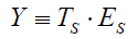
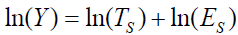
Symptoms as feelings of unpleasantness can be decomposed into true (TS) and error (ES) latent components. The error component is considered to represent random measurement error that is independent of the true symptom component. True and error symptom components are combined multiplicatively and expressed as
 ,
,
where Y is an observed continuous symptom response variable, and ≡ is interpreted as “defined as”. The implication is that Y is a derived variable caused by the co-joint effects of TS and ES. The symptom measurement model differs from the classical test score model in that true and error symptom components are combined multiplicatively rather than additively as in the neo-classic model [2, Tenet 1]. Tenet 1 refers to the first of 14 numbered tenets contained in Citation 2.
To be useful, symptoms must be symptomatic of an underlying pathology defined as the anatomic or dysfunctional manifestations of a disease or disorder denoted by a latent random variable P. The pathology measure P is considered to be decomposable into a true component 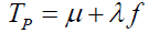 and an error component
 , with a neo-classical latent measurement model [2, Tenet 3]
 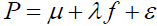 . The pathology true component and the symptom true component are linked by the exponential function
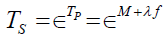 ,
,
where ∈is the base of the natural logarithms and μ +λ f is a pathology true score measure with μ = E(P) , λ =σP, and f the standardization of the P variable. The purpose is to establish a causal linkage between an underlying pathology and psychological feelings of unpleasantness. The linkage between error in the pathology measurement and error in symptom measurement is similarly depicted as  .
.
Upon substitution for TS and ES, the continuous symptom response variable Y can be expressed as
 ,
,
where μ +λ f and ε are as previously defined. In the absence of measurement error in the pathology variable P, ε =0 and the symptom response variable Y is unaffected, as ε 0 = 1. When ε < 0, the symptom response variable Y is attenuated, and conversely inflated when ε >0 as should be expected. As the standardized pathology variable  . Likewise, as
  . Consequently, Y>0, thereby avoiding the zero problem.
Logarithmic transformation
The logarithm has been referred to as the most useful arithmetic concept in science [9]. Its use in biology has been catalogued by Koch [10,11]. In psychology, logarithms form the basis of Fitt’s, Hick’s, and the Weber-Fechner Laws [12,13]. The log transformation applied to the multiplicative symptom response model is represented as
 ,
,
where ln(·) is the natural logarithm. The transformational effect is to convert the multiplicative symptom measurement model into a linear measurement model. Substituting the causal pathologic representation for TS and ES gives
 .
.
Scalar quantization
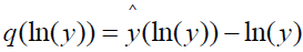
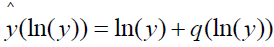
The continuous symptom response variable ln(Y) draws values from the real number line. However, symptom responses as conventionally scaled are restricted to integer values generally ranging from 1 to 5 or 7. This situation bears a remarkable similarity to the “analog” to “digital” conversion in signal theory. The process whereby an interval of analog signals is assigned a single scalar value is known in audio coding as scalar quantization [14]. Applied to symptoms measurement, experimental subjects select the integer value corresponding to the interval of ln(Y) containing their continuous ln(y) scores. The representation of a continuous symptom score ln(y) by an integer symptom scale representation  results in loss of information defined as
 ,
,
and referred to as quantization distortion or noise [14]. The rationale for the noise designation can be illustrated by rewriting the above equation as
 ,
,
which emphasizes the role of q(ln(y)) as add-on noise.
Scale coarseness
Coarseness in symptom scaling is a function of the number of scale benchmarks used to categorize the ln(Y) variable. The more benchmarks provided, the smaller the quantization error. Conversely, fewer benchmarks coarsen the scale and increase quantization noise. The effect of quantization noise is to introduce nonlinear and systematic error that serve to attenuate estimates of population covariance and correlation [15]. Because quantization noise is systematic, it should not be confused with measurement error which by definition is unsystematic variation. Aguinis, Pierce, and Culpepper [15] provide a table of correction factors for disattenuating the effects of scale coarseness on inter-scale correlations computed using benchmark integer values. Their corrections are incorporated into the Part II symptom scaling methodology herein proposed.
The log-normal distribution
As previously argued, the symptom measurement model can be expressed as lnY = μ +λ f +ε, which follows neo-classical test theory [2] in form with the exception that the observed variable Y is logarithmically transformed. As f and e in the pathology measurement model are defined as independent normally distributed random variables, ln Y as a weighted sum of normally distributed variables is itself normally distributed. Thus, Y can be said to be log-normally distributed with a two-parameter probability density function
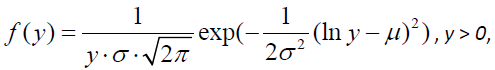
where μ is the location parameter and σ the scale parameter on a logarithmic scale. For a sample of size n, the parameters are estimated as 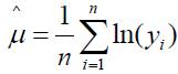 and
and 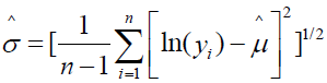 [16]. Sample parameter estimates are on a logarithmic scale as they are functions of the transformed value ln(yi), where i = i, 2, …, n. Depending upon parameter values, the log-normal distribution can range in shape from near normal to skewed. Location and scale parameter estimates on the logarithmic scale can also be directly obtained from the mean and variance of assumed normally distributed sample data according to the relations
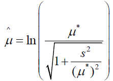
and
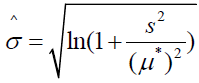 ,
,
where μ* and s are the mean and standard deviation, respectively, of the non-transformed original sample data [17].
Visual graphics as a decision tool
The most observable distinction between the neo-classical true score and the symptom measurement model is the proposed form of the data distribution. The neo-classical model assumes that the non-transformed data follow a normal distribution whereas the symptom model assumes a log-normal distribution. The extent of comparative fit can be visually examined by fitting a normal and a log-normal distribution to the histogram of the non-transformed Part II data and displaying the result as a graphical plot. A comparative fit index (CFI) can be computed for each distributional form according to the formula
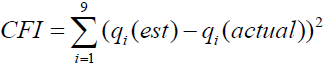 ,
,
where  is the estimated value for the 1%, 5%, 10%, 25%, 50%, 75%, 90%, 95%, and 99% quantiles of the normal or log-normal distribution and
 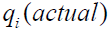 is the integer scale score corresponding to each quantile. The distribution with the lower CFI is judged to be the better fit. If the log-normal distribution is not the better fit, the hypothesis of a multiplicative measurement model is problematic. To log transform the original symptom scale data simply as a corrective for skewed data is subject to the scenario of misuses and misinterpretations as enumerated by Feng, Wang, Lu, and Tu [18]. Because the graphics procedure must be dynamic and able to operate in near real time as well as serving modeler’s immediate needs and interests, it has been described as dynamic-interactive by some authors [19].
Symptom scalability
A set of p symptom statements descriptive of unpleasant feelings associated with a target pathology is said to be scalable if there exists a standardized pathology measure f that is common to all p symptom statements. If so, then the log transformation of each symptom statement can be expressed as
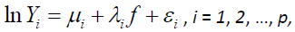
where  is the mean of an associated pathology measure
 is the standard deviation of Pi, and εi is the measurement error associated with Pi. The common presence of a single standardized pathology measure f underlying each of p log transformed symptoms implies that the p pathology measures are perfectly correlated and is the essence of the meaning of unidimensionality. For an extended discussion of unidimensionality in the context of true score theory, see [2, Tenet 5].
The hypothesis of scalability of a set of p symptom statements can be empirically tested by performing a confirmatory factor analysis (CFA) on the p x p correlation matrix of the log transformed values of Yi, i = 1, 2, … , p corrected for scale coarseness. For a more elaborative discussion, the reader is referred to [2, Tenet 11]. If the CFA model is judged to fit the log transformed data, the symptom statements can be considered to be scalable, with each statement contributing in varying degree to a single pathological measure. If the CFA fails to provide a satisfactory data fit, the p symptom statements should be regarded as nonscalable and further scale construction efforts abandoned for that set of symptom statements.
A comparative analysis
The distinction between human ability and human health measurement is most apparent when examining the comparative meaning of classical true score and true symptom. As both neo-classical true score and true symptom can be considered as mapping of an experimental probability space to real numbers [2], their difference must reside in the nature of the underlying generative experiment. For a more comprehensive discussion, the reader is referred to [2, Tenet 1]. Ability experiments as organized activity are designed to produce quantitative outcomes that differ in amount across a subject population. All subjects are assumed to possess this ability in some positive amount. Abilities as latent traits are relatively enduring over time. True implies that the latent trait scores are free of unsystematic measurement error.
Symptoms, in contrast, are self-reports of the presence of unpleasant states-of-being that impair human psychological and physiological functioning [20]. To be useful in a diagnostic and treatment capacity, symptoms must be symptomatic of some underlying biomedical causal agent, generally the presence of biological pathogens, inherent weakness, organ malfunctioning, or environmental stressors. When applied to mental functioning, epistemology in the United States generally takes the form of a biomedical model that posits that mental disorders are diseases of the brain amenable to pharmacological treatment [21]. This is not the case for traits which are posited to have a genetic causal framework making them relatively immutable to treatment [22].
Symptom pathology score
The initial step in symptoms research is to identify a target pathology of research interest. Measurement requires that p benchmarked statements considered as descriptive of manifest feelings emanating from the target pathology be developed and submitted to two-part modeling. A log-normal distribution is fitted to the histogram of Part II untransformed data for each statement and compared with the fit of a normal distribution.
If the log-normal is judged to be the better fit, Part II data are log transformed and a p x p correlation matrix computed and corrected for scale coarseness. A single-factor CFA is performed on the corrected correlation matrix. If the hypothesis of unidimensionality is sustained, the p statements can be said to be scalable and a single pathology score estimate  assigned to the jth symptomatic sample subject according to the formula
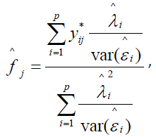
where  is the standardized log transformed observed score for the jth individual on the ith symptom statement and
  and
and are parameter estimates for the ith symptom statement obtained from performing an acceptable fitting CFA on the p x p correlation matrix of transformed Part II symptom data. In factor analytic terminology, this formulation is known as a Bartlett factor score [23].
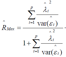
The reliability of the standardized latent pathology score  is defined as the squared canonical correlation between a maximally-weighted sum of p observed log transformed symptom scores and the standardized common pathology score variable f. This squared correlation is termed RMax, as it is the maximum squared correlation that can be obtained by choice of observed symptom weights, and is estimated as
A computer routine for two-part modeling
Due to the computational requirements of two-part modeling and the incorporation of computer graphics, a customized integrated execution routine is presented in Appendix A. The routine is written in the SAS® IML language. The routine accepts as input a SAS® data file containing only the numeric responses for p symptom statements scaled on a 5-point scale with no zero benchmark for a sample of N individuals. No other character or ID variables are permitted. Missing values are not allowed and if present must be imputed with an integer scale value prior to running. The routine accepts data files containing 4 to 10 symptom statements as variables. Users are asked to input the name of the SAS® library housing the data set; the assigned name for the SAS® data set; the number of variables contained in the specified data set; formatting notation related to number of variables; the choice as to whether or not to create data histograms; the choice as to normal or log-normal distributional form; the choice as to whether to save computed pathology scores; and the file name where pathology score estimates are to be saved. User input is checked for accuracy and the program terminated if an entry inconsistency is encountered.
Given no input inconsistencies, the routine begins by sorting sample observations into those who meet the asymptomatic criterion (having a p-item profile containing not less than p – 1 1s) and those who do not, considered as symptomatic. The asymptomatic subsample is deleted from further analytic consideration. Given the recommended starting options to create a histogram and a normal distribution, the routine runs SAS® Proc Univariate on each of the p symptomatic subsample variables and plots both a normal and a lognormal distributional fit on a single graph for visual comparison. Additionally, goodness-of-fit data are presented for nine quantiles. A utility for computation of a fit index based on quantiles is presented in Appendix B. Users are responsible for provision of quantile data to the fit index routine.
The Appendix A routine must be rerun with the “no histogram” option and log-normal distributional specification for each pathology to be scaled. As a result, the original data are log transformed. A p x p correlation matrix is computed, corrected for scale coarseness, and a CFA performed using SAS® Proc Calis. The routine outputs the distributional type; the symptomatic sample size; the asymptomatic sample size; CFA fit statistics; CFA parameters; RMax; pathology score mean; and pathology score uncorrected and corrected variance.
Exemplary Application of Two-part Modeling
Sampling procedure
The sample selected for exemplary two-part analysis is drawn from the National Survey of the Vietnam Generation (NSVG) Public Use Analysis File that contained the analysis variables from the National Vietnam Veterans Readjustment Study (NVVRS) [24]. The data source was selected because it represents the most comprehensive and documented sample of military veterans’ health outcomes ever assembled. In the NVVRS, study cohorts were selected via probability sampling by a two-stage national household design. An initial sample of 1187 male veterans who had served in the Vietnam theater was drawn from the NSVG Public Use Analysis File. Vietnam theater group veterans were targeted because they had the most direct combat experience. Males were targeted because females during the Vietnam War were prohibited from combat duty. Ten of the 1187 veterans each had more than five missing data values and were deleted, producing a final analysis sample of 1177 male Vietnam theater veterans. The final sample is considered a community sample, with community being defined as those male veterans who had served in the Vietnam theater of operations. As with community sampling in general, the proportion of the final sample suffering from PTSD as a dysfunctional pathology was unknown.
Sample data
PTSD symptom statements were drawn from the 35 items of the Mississippi Scale for Combat-Related Post-Traumatic Stress Disorder (M-PTSD) [25]. The M-PTSD items were scored on a 5-point Likert-type scale, adjusted for analytic purposes such that higher benchmark values always corresponded to greater dysfunctionality. No allowance was made for symptom absence. Item symptom statements were uniquely assigned to four pathologies identified from previous research as: Re-experiencing and Situational Avoidance; Withdrawal and Numbing; Arousal and Lack of Behavioral Control; Self- Persecution/Survivor Guilt [Schlenger WE (2014) PTSD symptoms research: A third generation approach]. Each of the pathologies and their associated symptom statements was hypothesized to constitute a unidimensional symptom measurement model. Prior to analysis, 23 missing values were imputed using the “hot deck” procedure [26], which has the advantage of imputing scale scores as whole numbers.
Scale purification
Each of the four hypothesized pathology scales was subject to tetrad-based purification using a six-step process suggested by Drewes [27]. As a result of purification, six items were deleted from the first pathology measurement model, five from the second, three from the third, and one from the fourth. The first pathology measurement model was renamed Re-experiencing and contained five subsidiary symptom statements. The second was renamed Withdrawal and contained six subsidiary symptom statements. The third was renamed Arousal and contained five subsidiary symptom statements. The fourth was renamed Self- Persecution and contained four subsidiary symptom statements. The four purified pathology models and their twenty component subsidiary statements are shown in Table 1.
| Item# |
Symptom statement |
CFI for normal distribution |
CFI for
log-normal distribution |
| Re-experiencing |
| Item1 |
I have nightmares of experience in military. |
2.230 |
0.363* |
| Item2 |
Dreams so real, I awake in cold sweat. |
3.110 |
0.823* |
| Item3 |
My daydreams are very real and frightening. |
2.561 |
0.763* |
| Item4 |
Unexpected noises make me jump. |
1.363 |
0.628* |
| Item5 |
Used alcohol or drugs to sleep or forget. |
4.016 |
0.617* |
| Withdrawal |
| Item1 |
Before I entered military, I had more friends. |
6.308 |
2.109* |
| Item2 |
I am able to get emotionally close to others. a |
0.913* |
1.007 |
| Item3 |
I still enjoy doing many things I used to enjoy. a |
1.385 |
0.519* |
| Item4 |
No one understands how I feel, not even my family. |
3.390 |
0.389* |
| Item5 |
I feel comfortable when I am in a crowd. a |
1.580 |
0.862* |
| Item6 |
My memory is as good as it ever was. a |
2.927 |
0.431* |
| Arousal |
| Item1 |
If pushed too far, I am likely to become violent. |
1.062* |
1.898 |
| Item2 |
The people who know me best are afraid of me. |
5.050 |
0.967* |
| Item3 |
I found it easy to keep my job since military. a |
3.897 |
1.636* |
| Item4 |
I am frightened of my urges. |
2.280 |
0.738* |
| Item5 |
I am an easy-going, even-tempered person. a |
1.063 |
0.617* |
| Self-Persecution |
| Item1 |
Reminded of my deeds, I wish I were dead. |
3.875 |
0.976* |
| Item2 |
Lately, I have felt like killing myself. |
5.516 |
0.992* |
| Item3 |
I wonder why I am still alive when others died. |
0.826* |
1.365 |
| Item4 |
I feel like I cannot go on. |
1.238 |
1.082* |
Note: CFI = Comparative fit index.
*A lower comparative fit index indicates a better fitting distribution.
aItem scoring reversal was employed.
Table 1: Four purified global symptoms, their component symptom statements, and comparative fit indices.
Results
Part I results
The Appendix A program was initially run with the “histogram” and “normal” option for each of the four pathology data sets. As a result, 20 separate histograms of untransformed symptomatic subject data were created. Histograms fitted with a normal and a log-normal distributional form are shown in Figure 1a-1e for Re-experiencing; Figure 2a-2f for Withdrawal; Figure 3a-3e for Arousal, and Figure 4a-4d for Self-Persecution. In the lower box for each figure, mean (Mu) and standard deviation (Sigma) for the original data are designated as Normal and mean (Zeta) and standard deviation (Sigma) for the log transformed data designated as Lognormal. Summary data for the non-transformed data fit by a normal distribution are contained in the upper side box. Visual examination shows that the histograms can be grouped into one of three types: those with frequencies clumping at lower scale values (L), those clumping at middle scale values (M), and those with frequencies tending to clump at higher scale values (H). Of the 20 symptom statements, 75% (15) fell into the L category, 20% (4) into the M category and 5% (1) into the H category. The interpretation is that for the majority of symptom statements, higher score values are endorsed by fewer and fewer symptomatic subjects, leading to a skewed distributional form.
Figure 1a: Histogram of a normal and a log-normal distribution for re-experiencing Item #1. The lower box shows mean (Mu) and standard deviation (Sigma) for the raw data and normal and zeta and sigma for the transformed data, respectively. Summary data for the non-transformed data are shown in the upper side box.
Figure 1b: Histogram of a normal and a log-normal distribution for re-experiencing Item #2. The lower box shows mean (Mu) and standard deviation (Sigma) for the raw data and normal and zeta and sigma for the transformed data, respectively. Summary data for the non-transformed data are shown in the upper side box.
Figure 1c: Histogram of a normal and a log-normal distribution for re-experiencing Item #3. The lower box shows mean (Mu) and standard deviation (Sigma) for the raw data and normal and zeta and sigma for the transformed data, respectively. Summary data for the non-transformed data are shown in the upper side box.
Figure 1d: Histogram of a normal and a log-normal distribution for re-experiencing Item #4. The lower box shows mean (Mu) and standard deviation (Sigma) for the raw data and normal and zeta and sigma for the transformed data, respectively. Summary data for the non-transformed data are shown in the upper side box.
Figure 1e: Histogram of a normal and a log-normal distribution for re-experiencing Item #5. The lower box shows mean (Mu) and standard deviation (Sigma) for the raw data and normal and zeta and sigma for the transformed data, respectively. Summary data for the non-transformed data are shown in the upper side box.
Figure 2a: Histogram of a normal and a log-normal distribution for withdrawal Item #1. The lower box shows mean (Mu) and standard deviation (Sigma) for the raw data and normal and zeta and sigma for the transformed data, respectively. Summary data for the non-transformed data are shown in the upper side box.
Figure 2b: Histogram of a normal and a log-normal distribution for withdrawal Item #2. The lower box shows mean (Mu) and standard deviation (Sigma) for the raw data and normal and zeta and sigma for the transformed data, respectively. Summary data for the non-transformed data are shown in the upper side box.
Figure 2c: Histogram of a normal and a log-normal distribution for withdrawal Item #3. The lower box shows mean (Mu) and standard deviation (Sigma) for the raw data and normal and zeta and sigma for the transformed data, respectively. Summary data for the non-transformed data are shown in the upper side box.
Figure 2d: Histogram of a normal and a log-normal distribution for withdrawal Item #4. The lower box shows mean (Mu) and standard deviation (Sigma) for the raw data and normal and zeta and sigma for the transformed data, respectively. Summary data for the non-transformed data are shown in the upper side box.
Figure 2e: Histogram of a normal and a log-normal distribution for withdrawal Item #5. The lower box shows mean (Mu) and standard deviation (Sigma) for the raw data and normal and zeta and sigma for the transformed data, respectively. Summary data for the non-transformed data are shown in the upper side box.
Figure 2f: Histogram of a normal and a log-normal distribution for withdrawal Item #6. The lower box shows mean (Mu) and standard deviation (Sigma) for the raw data and normal and zeta and sigma for the transformed data, respectively. Summary data for the non-transformed data are shown in the upper side box.
Figure 3a: Histogram of a normal and a log-normal distribution for arousal Item #1. The lower box shows mean (Mu) and standard deviation (Sigma) for the raw data and normal and zeta and sigma for the transformed data, respectively. Summary data for the non-transformed data are shown in the upper side box.
Figure 3b: Histogram of a normal and a log-normal distribution for arousal Item #2. The lower box shows mean (Mu) and standard deviation (Sigma) for the raw data and normal and zeta and sigma for the transformed data, respectively. Summary data for the non-transformed data are shown in the upper side box.
Figure 3c: Histogram of a normal and a log-normal distribution for arousal Item #3. The lower box shows mean (Mu) and standard deviation (Sigma) for the raw data and normal and zeta and sigma for the transformed data, respectively. Summary data for the non-transformed data are shown in the upper side box.
Figure 3d: Histogram of a normal and a log-normal distribution for arousal Item #4. The lower box shows mean (Mu) and standard deviation (Sigma) for the raw data and normal and zeta and sigma for the transformed data, respectively. Summary data for the non-transformed data are shown in the upper side box.
Figure 3e: Histogram of a normal and a log-normal distribution for arousal Item #5. The lower box shows mean (Mu) and standard deviation (Sigma) for the raw data and normal and zeta and sigma for the transformed data, respectively. Summary data for the non-transformed data are shown in the upper side box.
Figure 4a: Histogram of a normal and a log-normal distribution for self-persecution Item #1. The lower box shows mean (Mu) and standard deviation (Sigma) for the raw data and normal and zeta and sigma for the transformed data, respectively. Summary data for the non-transformed data are shown in the upper side box.
Figure 4b: Histogram of a normal and a log-normal distribution for self-persecution Item #2. The lower box shows mean (Mu) and standard deviation (Sigma) for the raw data and normal and zeta and sigma for the transformed data, respectively. Summary data for the non-transformed data are shown in the upper side box.
Figure 4c: Histogram of a normal and a log-normal distribution for self-persecution Item #3. The lower box shows mean (Mu) and standard deviation (Sigma) for the raw data and normal and zeta and sigma for the transformed data, respectively. Summary data for the non-transformed data are shown in the upper side box.
Figure 4d: Histogram of a normal and a log-normal distribution for self-persecution Item #4. The lower box shows mean (Mu) and standard deviation (Sigma) for the raw data and normal and zeta and sigma for the transformed data, respectively. Summary data for the non-transformed data are shown in the upper side box.
Separate fit indices were computed for each histogram using the program in Appendix B for the normal and for the log-normal distribution for each of the 20 symptom statements. The 99th quantile was excluded from the computation due to erratic influence on the log-normal fit index. Comparative results are shown in Table 1, where a lower index indicates a better fitting distribution. The log-normal distributional form exhibited a lower fit index for 17 of the 20 symptom statements. The normal form provided a better fit for Figures 2b, 3a and 4c, accounting for three of the four statements with mid-scale distributional clumping. The histogram as shown in Figure 1d, although exhibiting mid-scale clumping, is better fit by a log-normal than a normal distribution.
The comparative fit indices reported in Table 1 are univariate statistics and hence fail to take intra-pathology symptom correlation into account. A multivariate comparative index was computed based on the fact that the Mahalanobis d-squared statistic for a multi-normal distribution is chi-squared distributed [28]. The squared distance between estimated and observed vectors of 1%, 5%, 10%, 25%, 50%, 75%, 90% and 95% quantiles was computed for the original and log transformed symptomatic sub-sample data. Comparative results show 2.797 for the normal vs. 1.879 for the log transformation for Re-experiencing; 4.608 for the normal vs. 0.833 for the log transformation for Withdrawal; 2.252 for the normal vs. 0.861 for the log transformation for Arousal; and 6.256 for the normal vs. 0.954 for the log transformation for Self-Persecution. The log transformation produced a better comparative fit for all pathology measurement models, thereby supporting the hypothesis of multiplicative combination of symptom true and error components. A routine for computing the multivariate comparative fit index is presented in Appendix C.
Sample size designated as N in the Summary Statistics histogram boxes ranged from 846 for Re-experiencing, 1133 for Withdrawal, 980 for Arousal, and 310 for Self-persecution. In the context of two-part modeling, sample size is the estimated number of symptomatic individuals and can be construed as a prevalence measure. Accordingly, the four pathology measures ranked by prevalence are Withdrawal, Arousal, Re-experencing, and Self-persecution. Self-persecution is an outlier with 1177 – 310 = 867 veterans meeting the asymptomatic criterion.
Part II results
Computer outputs generated by rerunning the Appendix A program with the “no histogram” and “log-normal” options are presented in the supplementary file: Statistical Output A for Re-experiencing, Statistical Output B for Withdrawal, Statistical Output C for Arousal, and Statistical Output D for Self-Persecution. Each statistical output is structured so as to provide users with summary information as to symptomatic and asymptomatic sample sizes, confirmatory factor analysis (CFA) fit statistics, standardized CFA factor loadings and accompanying standard error, residual error variance and accompanying standard error, and the RMax reliability estimate.
Acceptance of the hypothesis of unidimensionality is dependent upon whether or not CFA produces an acceptable fit. Model fit is a subjective determination dependent in part on the probability of obtaining a chi square value greater than the observed value (P-Value); conventional fit indices (CFI and TLI); and root mean square of approximation (RMSEA). For a reasonably good-fitting CFA model, P-Value should be greater than 0.001; CFI and TLI should be greater than 0.90; and RMSEA should be less than or equal to 0.05 [29]. Judging from the results as shown in Statistical Outputs A-D, the hypothesis of unidimensionality is confirmed for Re-experiencing, Withdrawal, and Arousal and rejected for Self-persecution based on P-value<0.001, CFI<0.90; TLI<0.90, and RMSEA>0.05. The implication is that the symptom statements assigned to Re-experiencing, Withdrawal, and Arousal, respectively, can be combined into a weighted sum as each statement measures the same underlying pathology. Component statements assigned to Self-persecution cannot be combined, as the CFA results do not support the hypothesis of a common pathology underlying each of the four component symptom statements.
The results designated as factor loadings in Statistical Outputs A-D represent the relative importance of each observed symptom statement in the measurement of the underlying standardized pathology measurement. Symptom statements with a factor loading >0.60 are referred to as marker symptoms as they make the major contribution to the pathology score. Because marker symptoms make the major measurement contribution, they are useful in furthering understanding of underlying causes.
The standardized factor loadings in Statistical Output A show two feeling statements that qualify as marker variables: “I have nightmares of experience in military.” with a loading of 0.751 and “Dreams so real, I awake in cold sweat.” with a loading of 0.844. Both symptom statements pertain to dreams as the re-experiencing modality. Statistical Output B indicates two withdrawal statements as marker variables: “I still enjoy doing many things I used to enjoy.” with a loading of 0.629 and “No one understands how I feel, not even my family.” with a loading of 0.654. Withdrawal as behavioral dysfunctionality appears to be manifested in feelings of alienation in a civilian world in spite of continued enjoyment of many prior civilian activities. Arousal (Statistical Output C) is marked by a single symptom statement: “The people who know me best are afraid of me.” with a loading of 0.762. This suggests that awareness of the familial and societal consequences of unmanageable agitated behavior is a central facet of Arousal. Factor loadings for Self-persecution have no interpretation as markers in that the hypothesis that each symptom statement manifests the same underlying pathology is rejected.
Acceptance of the unidimensionality hypothesis does not necessarily imply that all manifest symptom statements are equally reliable. Statement reliability is measured by the square of the standardized factor loadings. Reliabilities for the five statements manifesting Re-experiencing are: 0.564, 0.712, 0.265, 0.243, and 0.203. Reliabilities for the six statements manifesting Withdrawal are 0.295, 0.126, 0.396, 0.427, 0.233, and 0.276. Reliabilities for the five statements manifesting Arousal are 0.278, 0.580, 0.081, 0.346, and 0.155. Reliability estimates for Self-persecution statements are meaningless in the absence of a common pathology measure.
The range of manifest symptom reliabilities, (0.712-0.203) for Re-experiencing, (0.427-0.126) for Withdrawal, and (0.580- 0.081) for Arousal attest to the multi-faceted complexity of PTSD pathologies [30]. No single symptom statement has sufficient reliability to serve as a sole proxy for the common pathology. Yet each has the potential to make a unique contribution. A promising approach is to use a weighted combination of all constituent manifest symptoms to predict a pathology score. The square of the multiple-regression coefficient is RMax, as previously defined. Estimated RMax values are given in Statistical Output A-D as 0.825 for Re-experiencing, 0.726 for Withdrawal, and 0.720 for Arousal.
The difference between RMax and the square of the largest component factor loading represents the contribution of the remaining symptom statements to latent pathology prediction. For the Re-experiencing component, the remaining four statements account for (0.825–0.712) x 100% = 11.3% of the pathology score variance; for Withdrawal, the remaining five statements account for (0.726–0.427) x 100% = 29.9% of Withdrawal variance; and for Arousal, the remaining four statements account for an additional (0.720–0.580) x 100% = 14% of Arousal variance. The larger residual contribution for Withdrawal is probably due to an additional symptom statement. The evidence-based conclusion is that the remaining statements in each component measurement model make a significant contribution to pathology score measurement and should be retained in the model. No conclusions can be drawn for Self-persecution, as the measurement model failed the CFA test for unidimensionality.
The standardized beta coefficient  for the ith manifest symptom statement, i = 1, 2, … p, is estimated as
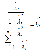 ,
,
where  is the estimated standardized factor loading for the ith manifest symptom statement. Estimated standardized beta coefficients for the five symptom statements for Re-experiencing are BR = {0.366 0.624 0.149 0.138 0.120}; for the six Withdrawal statements BW = {0.291 0.153 0.393 0.431 0.237 0.274}; and BA = {0.284 0.706 0.121 0.350 0.182} for the five Arousal statements. Marker variables have the highest beta weights for each of the three PTSD components.
A latent pathology score is estimated for the jth subject as a weighted standardized score according to
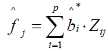 , where is as previously defined and Zij is a profile of standardized log transformed symptom scores. Note that the weighted score interpretation is equivalent to the Bartlett factor score as previously defined. Depending upon user discretion, the Appendix A routine can compute individual subject latent pathology scores and save as a SAS® file in a designated library.
Conclusion
Statistical analyses with latent pathology scores
For analysis purposes, latent pathology scores can be treated as if they were empirical variables. Means, variances, covariance, and correlations can be computed using conventional formulae. This allows researchers to establish inter-correlations among a set of differential pathologies; to use pathology scores as predictors of external health-related criteria variables or conversely external health-related variables as predictors of single or multiple pathology scores; or to perform cluster or factor analyses to determine the dimensionality of a correlation matrix of selected pathologies.
There is, however, an important caveat to bear in mind. Latent pathology scores, more generally known as Bartlett factor scores, are weighted summations of standardized log transformed observed scale scores. Accordingly, the variance of pathology scores contains a contribution due to residual error variance. This contribution serves to inflate the computed variance estimate resulting in an upward bias. Fortunately, the population variance of standardized Bartlett factor scores fB can be expressed as
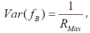
where RMax is as previously defined (see Appendix D for proof). Thus, Var(fB) = 1 only when RMax = 1, which implies perfect scale reliability. As RMax decreases, Var(fB) increases due to presence of measurement error in the transformed observed symptom statements. Therefore, multiplication of Var(fB) by RMax as a correction yields unity which is the unbiased population value. This relation holds at the population level and may vary somewhat due to sampling error.
Computer output for the three PTSD components shown in Statistical Outputs A-D include Bartlett score means, Bartlett score variance uncorrected, and Bartlett score corrected variance. Due to standardization of profile scores, Bartlett score means were near zero for all three PTSD components. Bartlett score uncorrected variance is 1.142 for Re-experiencing, 1.289 for Withdrawal, and 1.319 for Arousal. The fact that all uncorrected score variance estimates exceed unity is indicative of the presence of measurement error. When corrected by multiplication by component RMax, component score corrected variance estimate is 0.942 for Re-experiencing, 0.936 for Withdrawal, and 0.949 for Arousal. All corrected variance estimates are near the upper boundary of unity.
Whereas uncorrected Bartlett score variance is subject to the biasing effects of measurement error, Bartlett score covariance is not (see Appendix D for proof). Correlation between Bartlett scores fB(i) and fB(j), interpreted as scores on separate pathologies, is defined as
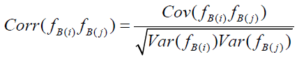 .
.
But as previously discussed,  and
and  are inflated due to presence of measurement error, serving to attenuate
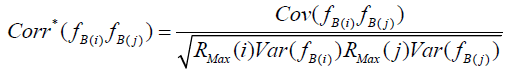
  . Correction for attenuation is accomplished by multiplication of each uncorrected Bartlett score variance by its associated RMax
 ,
,
where  is the disattenuated factor score correlation. By incorporating the definition of correlation, the pair-wise factor score correction for attenuation can be rewritten as
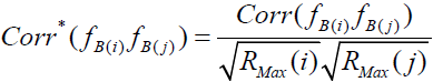 ,
,
which is the factor score extension of Spearman’s correction for attenuation [31].
Sample size is at issue as the number of symptomatic subjects varies by component pathology. For the PTSD example, the symptomatic sample size was 846 for Re-experiencing, 1133 for Withdrawal, and 980 for Arousal. The Appendix A routine designates asymptomatic subjects as missing values in the computation and storage of Bartlett factor scores. This has the advantage of maintaining a constant sample size across component factors (N = 1177 for the PTSD example).
Remaining at issue is how to handle missing values. The simplest approach is to compute pair-wise correlations using only those observations with non-missing factor scores on both pathology factors. While simple, the pair-wise approach has the disadvantage that Bartlett score inter-correlations may be based on different subjects depending upon the selected factor pair. Correlations based on different sample sizes and subject composition poses serious statistical problems for analyses requiring a k x k (k>2) dimensional correlation matrix. Consequently, a recommended solution is to keep all observations that have no missing values on the k Bartlett scores and to drop all others. By so doing, all k(k-1)/2 pair-wise correlations are based on the same sample and can be estimated by conventional means. More sophisticated missing value imputation is unsuitable either due to non-random missing value assignment or lack of external covariates to permit missing value prediction.
Implementation of the recommended procedure requires that the k Bartlett score files created by sequential running of the Appendix A utility for each component factor be merged into a single file. The k factors in the merged file must then be inter-correlated with the requirement that all retained sample observations contain no missing values. In SAS® Version 9.4 [32], this is accomplished by the following code:
data in.PTSD_merge;
merge in.PTSD1_BS
in.PTSD2_BS(rename=(v1=v2))
in.PTSD3_BS(rename=(v1=v3));
run;
proc corr data=in.PTSD_merge nomiss;
run;
File names are those used in analysis of the PTSD data. File naming conventions are at the user discretion but must be the same as those used in each of the separate analyses. Variables must be renamed sequentially in the merged file, as by default the Bartlett score variable in each merged file is named v1.
Running the above program produces attenuated correlations. Correlations are corrected for attenuation by dividing each off-diagonal attenuated correlation by the square root of the product of the RMax for each contributing factor. In the following matrix, uncorrected correlations for the three PTSD pathologies are shown above the diagonal and corrected correlations below the diagonal.
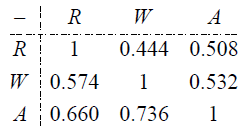
Each correlation is based on a sample size of 766, which is the number of observations with no missing values on all three pathology scores. For the PTSD example, 766 out of 1177 subjects qualified as symptomatic on each of the three PTSD pathology factors. Withdrawal and Arousal exhibit the highest and Withdrawal and Reexperiencing the lowest pair-wise correlations.
Symptoms Research – A Sequential Approach
Symptoms as latent variables. The premise of this paper is that neo-true score theory [2] can be meaningfully applied to psychopathological symptoms measurement. At the core is the axiom that an observed symptom score can be decomposed into a true-score and an error-score component. True and error symptom score components are each non-observable and assigned the status of latent variables. Error symptom latent scores are independent of true symptom scores, with the implication that true symptom scores are measured error free.
The definition of symptom true and error scores differ from that used in neo-classic test score theory. For mental ability test scores X, true score is defined as 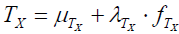 , where
  is the population true score mean, λTx is the population true score standard deviation, and
  is the standardized population true score [2, Tenet 5]. In contrast, for symptom score Y , true symptom score TY is a derived rather than a primary variable and is expressed as
 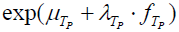 , where exp is the base of the natural logarithms and
  is the true component TP of an underlying causal pathology measure P. Exponentiation ensures that as the standardized pathology measure
  ,
,  . Similarly, untransformed symptom error is expressed as
 where εP is the error component of P, thereby ensuring that
  as
as  . Consequently, the zeroproblem is skirted, as Y >0.
True score model differences. In neo-classical test theory, true and error score components are additively combined [2]. For an observed symptom random variable Y , true and error components are instead hypothesized to be multiplicatively combined as Y = TY·EY By defining  and
and  ,
,  under the assumption that the pathology P score components are additively combined. Consequently, ln(Y) = P under the multiplicative combination of true and error symptom components so defined. If the pathology variable P is normally distributed, then by definitional equivalence, so must ln(Y). The distributional form wherein the log of a variable is normally distributed is known as a log-normal distribution. The normal distribution has the property that if two variables are each normally distributed, then their sum is also normally distributed. The log-normal distribution also shares this feature—if true and error components are each log-normally distributed, then their sum is also log-normally distributed. The normal and the log-normal are the only well-known statistical distributions with this essential modeling property.
This leaves symptoms researchers with two options as to measurement models—additive or multiplicative. There is recognition in the literature that symptoms may be multiplicative [33]. Fortunately, each type has a recognizable visual signature. For the normal bell curve, observations cluster symmetrically around the mean. The odds of a symptom score being less than one standard deviation below the mean are approximately 1 in 6.3 and equals the odds of a symptom score being more than one standard deviation above the means. The odds increase exponentially as the distance below or above the mean increases [34]. In contrast, for the log-normal distribution, the mass of the probability density function is disproportionally grouped at the lower or higher end of the scale resulting in a skewed distribution. Skewness is visually illustrated in Figure 1b, the second symptom statement for the Re-experiencing pathology. For a normal distribution fit to that data, the probability of a scale value less than 2 is 0.510, as contrasted with 0.611 for the log-normal distribution fit to the same data. The increase in probability is due to clumping of observations at lower scale values.
The hypothesis that system true and error components are best considered to be multiplicatively combined is tested by the multivariate CFI presented in Appendix C. A lower CFI for the log-normal distribution is confirmatory evidence for the multiplicative assertion. A lower CFI for the normal distribution suggests that Part II multivariate symptom data fail to support a multiplicative measurement model.
Modeling in symptoms research. For symptoms researchers, a legitimate question is: Why model? Conventional practice tends to treat individual symptom statements as bona fide symptom entities. What is often overlooked is that symptoms as reported unpleasant feelings occur within the broader context of individual subjective experience [33]. Symptoms are communicated by self-reports of those experiencing them. As such, they are subject to the vagaries of social communication [35]. Meaning assigned to physical sensations may well vary by demographic as well as individual factors. Variation introduced by systematic demographic characteristics can be controlled by population sampling. Individual factors, however, encompass non-systematic variability due to temporal situational states of mind [1]. Non-systematic effects are considered to occur randomly and are collectively referred to as measurement error.
If individual symptom statements are to have clinical utility, they must measure the systematic effects of causal pathologies. These systematic effects are referred to as true scores in classic measurement theory. True score contribution varies across symptom statements as reflected by differential statement reliability. It is quite possible for individual symptom statements to measure mainly random error, contradicting the prevalent supposition that statements are error free.
True scores as a measure of systemic effects vary in degree of uniqueness. At one extreme, each symptom statement has a unique true score indicating that each statement measures a different pathological entity. In this case, there are as many pathologies as there are symptom statements. The counter condition is that all symptom statements in the modeling domain measure a common latent pathology, a condition herein referred to as unidimensionality. Observable symptom statements are herein defined as containing both true and error measurement effects multiplicatively combined.
The classic means of dealing with error-prone measurement is summation over a large number of observed score replications [36]. The supporting rationale is that measurement error, being random, can be expected to be self-canceling over a large number of measurement instances. Whereas the logic with respect to error has stood the test of time, the meaning of a sum of error-free true symptom components is not so clear-cut. If each true variable is unique to a single symptom statement, the sum over p statements is a mishmash of unrelated pathological effects defying a meaningful interpretation. It is only when each symptom statement assigns an identical standardized true score to an individual subject, i.e., a defining property of unidimensionality, that meaning emerges.
The unidimensionality of a set of p symptom statements is empirically verifiable by running a single-factor confirmatory factor analysis (CFA) on the p x p correlation matrix. If the hypothesis of unidimensionality is sustained, symptoms researchers are faced with attaching meaning to the common variable. Standardized true score is a possibility but emphasizes mainly the error-free nature. Factor is a tempting choice but focuses more on dimensionality than function. Syndrome as a collection of signs and symptoms characteristic of a known pathological condition [37] appears a better option but shifts attention to the collectivity and away from the function served. The convention endorsed in this paper is to emphasize the core measurement function—mapping of the amount of quantified symptom unpleasantness due to causal pathologies to the real number line. For a more detailed discussion, please refer to [2, Tenet 1] which differs in application only to the extent that mental traits as opposed to mental states are addressed.
Unreliability of individual symptom statements attenuates the measurement of felt unpleasantness due to pathological conditions. The remedy is to use the p observed symptom statements as independent variables in a multiple regression model to predict pathology scores. The square of the multiple correlation coefficient is referred to as RMax and is the maximum correlation that can be obtained by weighting individual statements. Under the supposition that all p statements have some reliability, RMax will exceed the reliability of any symptom statement considered in isolation. This gain epitomizes the system adage that the whole is greater than the sum of its parts and constitutes the major rationale for symptoms modeling.
Summary Remarks
A case for a two-part symptoms modeling procedure as a means of dealing with the zero-problem inherent in community sampling has been made. The procedure assumes the pre-existence of a pool of p statements descriptive of adverse feelings considered to be caused by a target pathology. Statements may be drawn from existing scales or constructed to reflect contemporary research results, theories, or clinical intuition. Statements are self-rated on a five-point scale, preferably with a severity, duration, or frequency metric common to all statements. Whatever the metric, the leftmost benchmark is generally indicative of minimal unpleasantness.
Central to the zero-problem is the not-so-remote possibility that a portion of a community sample may be asymptomatic, thereby constituting a zero class. As there is generally no scale provision for symptom absence, it is reasonable to suspect that zero-class members will likely gravitate to the left-most response category thereby creating a skewed distribution. Part I of the proposed two-part model operationally defines zero-class members as those respondents whose response profile contains at least p – 1 leftmost category responses. Respondents whose profiles qualify are deleted from further modeling consideration.
Unlike modeling procedures that assume a normal distribution, the proposed two-part procedure presumes a log-normal Part II data distribution to ensure positive symptom amounts. Dependence on the normal curve implies acceptance of an additive measurement model which produces a symmetrical response distribution. The rationale for log-normal, in contrast, employs a multiplicative measurement mechanism and produces distributional shapes varying from near normal to extreme skewness.
To facilitate visual comparison, the computerized procedure fits both a normal and a log-normal distribution to the symptomatic sample histogram for each of the p symptom statements. A univariate and a multivariate comparative fit statistic measuring the agreement between observed and predicted quantiles are computed from procedural output. Acceptance of the multiplicative hypothesis is conditional on the log-normal being the better fit. If the multiplicative hypothesis is sustained, sample data are logarithmically transformed prior to Part II analysis.
Part II analyses consist of testing the unidimensionality hypothesis by running and reporting CFA results. Prior to analysis, the p x p correlation matrix is corrected for attenuation due to scale coarseness. Scalar quantization is offered as the means of analog-to-digital conversion. Standard fit indices and heuristics for their interpretation are provided to aid users in ascertaining CFA model fit. The RMax coefficient is computed. Users should be reminded that its use is conditional on the unidimensionality hypothesis being sustained.
Standardized Bartlett pathology scores are computed, with users having the option of storing for future use. Bartlett scores have the advantage of incorporating the collective measurement contribution of p manifest symptom statements into a single pathology score. Bartlett scores can be used as if they were empirically obtained, with the singular exception that their sample variance is inflated due to the presence of measurement error in the component manifest statements.
By the sequential application of two-part modeling, Bartlett scores for a community sample can be formulated for each of k target pathologies. Researchers should avoid overlapping identical symptom statements across the k pathology scales. To do so would allow a symptom statement to manifest multiple pathologies thereby violating the unidimensional scaling requirement. A k x k correlation matrix with no missing values can be computed, corrected for attenuation, and used as input for a variety of multi-variable statistical applications. Hopefully, two-part modeling will enhance the capability of symptoms researchers to alleviate human suffering.
Author Note
Donald W. Drewes, Chia-Lin Ho, and William E. Schlenger, Department of Psychology, NC State University.
Chia-Lin Ho is now at BB&T Leadership Institute; William E. Schlenger is now retired.
Correspondence concerning this article should be addressed to Donald W. Drewes, Department of Psychology, NC State University, Raleigh, NC 27695.
References
- Steyer R, Mayer A, Geiser C, Cole DA (2015) A theory of states and traits: revised. Annu Rev Clin Psychol 11: 71-98.
- Drewes DW (2017) Neo-classical test theory: a modernization. Acta Psychopathol 3: 68.
- Kaplan R (1999) The nothing that is: a natural history of zero. New York: Oxford University Press, p: 240.
- https://www.verywellmind.com/community-sample-425241
- Bollen KA (1989) Structural equations with latent variables. New York: Wiley, p: 528.
- Kim YK, Muthén BO (2009) Two-part factor mixture modeling: application to an aggressive behavior measurement instrument. Struct Equ Modeling 16: 602-624.
- Olsen MK, Schafer JL (2001) Two-part random-effects model for semicontinuous longitudinal data. J Am Stat Assoc 96: 730-745.
- Neelon B, O’Malley AJ, Smith VA (2016) Modeling zero-modified count and semicontinuous data in health services research Part 1: background and overview. Stat Med 35: 5070-5093.
- https://www.physics.uoguelph.ca/tutorials/LOG/
- Koch AL (1966) The logarithm in biology 1. mechanisms generating the log-normal distribution exactly. J Theoret Biol 12: 276-290.
- Koch AL (1969) The logarithm in biology II. distributions simulating the log-normal. J Theoret Biol 23: 251-268.
- https://ta1clogarithms.blogspot.com/2011/07/logarithms-in-psychology.html
- https://logarithmsandpsychology.blogspot.com/
- You Y (2010) Audio coding: theory and application (chapter 2). Springer Science & Business Media; p: 291.
- Aguinis H, Pierce CA, Culpepper SA (2009) Scale coarseness as a methodological artifact: correcting correlation coefficients attenuated from using coarse scales. Organ Res Methods 12: 623-652.
- Limpert E, Stahel WA, Abbt M (2001) Log-normal distributions across the sciences: keys and clues. Bioscience 51: 341-352.
- https://en.wikipedia.org/w/index.php?title=Log-normal_distribution&printable=yes
- Feng C, Wang H, Lu N, Tu X (2012) Log transformation: application and interpretation in biomedical research. Stat Med 32: 230-239.
- Valero-Mora P, Ledesma R (2014) Dynamic-interactive graphics for statistics (26 years later). Rev Colomb Estad 37: 247-260.
- Lenz ER, Pugh LC, Milligan RA, Gift A, Suppe F (1997) The middle-range theory of unpleasant symptoms: an update. ANS Adv Nurs Sci 19: 14-27.
- Deacon BJ (2013) The biomedical model of mental disorder: a critical analysis of its validity, utility, and effects on psychotherapy research. Clin Psychol Rev 33: 846-861.
- Chaplin WF, John OP, Goldberg LR (1988) Conceptions of states and traits: dimensional attributes with ideals as prototypes. J Pers Soc Psychol 54: 541-557.
- https://pareonline.net/pdf/v14n20.pdf
- Kulka RA, Schlenger WE, Fairbank JA, Hough RL, Jordan BK, et al. (1990) Trauma and the Vietnam war generation: report of findings from the national Vietnam veterans readjustment study. New York: Brunner/Mazel, p: 322.
- Keane TM, Caddell JM, Taylor KL (1988) Mississippi scale for combat-related post-traumatic stress disorder: three studies in reliability and validity. J Consult Clin Psychol 56: 85-90.
- Korn EL, Graubard BL (1999) Sample weights and imputation. Analysis of health surveys. New York: Wiley, pp: 183-184.
- Drewes DW (2009) Subject-centered scalability: The sine qua non of summated ratings. Psychol Methods 14: 258-274.
- https://en.wikipedia.org/wiki/Mahalanobis_distance
- Muthén BO (1998-2004) Mplus technical appendices (Appendix 5). Los Angles: Muthén & Muthén.
- Galatzer-Levy IR, Bryant RA (2013) 636,120 ways to have posttraumatic stress disorder. Perspect Psychol Sci 8: 651-662.
- Allen MJ, Yen WM (1979/2002) Introduction to measurement theory. Long Grove, IL: Waveland Press, Inc, p: 310.
- https://www.sas.com/en_in/software/sas9.html
- Armstrong TS (2003) Symptoms experience: a concept analysis. Oncol Nurs Forum 30: 601-606.
- Taleb NN (2007) The black swan: the impact of the highly improbable. New York: Random House, p: 366.
- Luhmann N (2013) Introduction to systems theory. Malden, MA: Polity Press, p: 300.
- Eisenhart C (1983) Laws of error I: development of the concept. In: Encyclopedia of statistical science (Kotz S, Johnson NL Edn). Toronto: Wiley, 4: 530-547.
- https://en.wikipedia.org/w/index.php?title=Syndrome&printable=yes
Appendix A
TITLE: A computer routine to execute two-part modeling
REQUIREMENTS: SAS/STAT Version 9.4 & SAS/IML Version 9.4
DISCLAIMER: This utility is provided by the authors as a service to Acta Psychopathologica readers. There are no warranties, expressed or implied, as to the accuracy of the code provided herein.
CODE:
/*Routine to extract a dysfunctional sample from a mixture population of functional and dysfunctional sub-populations.*/
/*Items are assumed to be quantized to five digital values with 1 representing the absence or near absence of dysfunctionality.*/
/*Observations are classified as dysfunctional if all p-items responses are greater than 1 or a unit response is given to only one item.*/
/*Scores for functional observations are treated as missing.*/
/*A sample of observations meeting the dysfunctionality criterion is created and a p x p correlation matrix computed.*/
/*The correlation matrix is corrected for attenuation due to quantization.*/
/*A single-factor CFA is performed on the corrected correlation matrix and Bartlett factor scores computed and saved.*/
/*User note: Enter the SAS library where the input mixture file is stored.*/
/*User note: Do NOT change ‘in’ libname.*/
libname in "H:\My SAS Data Files\V9.1";s
/*User note: Enter the file name of the input mixture file.*/
%let filename = PTSD_dim1;
/*User note: Routine restricts number of variables per scale to not less than four and not more than ten.*/
/*User note: Please enter the number of manifest variables.*/
%let num_vars = 5;
%let vars_num = 'v1-v5';
%let var_num = v1:v5;
%let name_vars = 'v1':'v5';
/*User note: User has choice as to whether to create item histograms. If not, enter 1, if yes enter 2.*/
%let hist_comp = 2;
/*User note: User has choice as to normal or lognormal distributional form. If normal, enter 1. If lognormal, enter 2.*/
%let dist = 1;
/*User note: User has option of saving corrected Bartlett scores. If not,enter 1, if yes enter 2.*/
%let BS_save = 1;
/*User note: Enter name of file where Bartlett scores are to be saved. File will be stored in above designated SAS library.*/
%let B_scores = PTSD1_BS;
/* **************************Do not alter code beyond this point ****************************************************** */
proc iml;
choice = &hist_comp;
dist_kind = &dist;
/*Get original data matrix.*/
use in.&filename;
read ALL var _NUM_ into X;
close in.&filename;
N = nrow(X);
p = ncol(X);
if p ^= &num_vars then
do;
print "Number of file variables does not agree with user designation.";
abort;
end;
if (p <4) | (p > 10) then
do;
print "Number of scale variables outside permissible range.";
abort;
end;
/*Compute combinations of p items.*/
a = 1:p;
do i = 1 to p;
if i = 1 then
do;
k1 = allcomb(p,a[1,i]);
call sort(k1,1:i);
end;
else
if i = 2 then
do;
k2 = allcomb(p,a[1,i]);
call sort(k2,1:i);
end;
else
if i = 3 then
do;
k3 = allcomb(p,a[1,i]);
call sort(k3,1:i);
end;
else
if i = 4 then
do;
k4 = allcomb(p,a[1,i]);
call sort(k4,1:i);
end;
else
if i = 5 then
do;
k5 = allcomb(p,a[1,i]);
call sort(k5,1:i);
end;
else
if i = 6 then
do;
k6 = allcomb(p,a[1,i]);
call sort(k6,1:i);
end;
else
if i = 7 then
do;
k7 = allcomb(p,a[1,i]);
call sort(k7,1:i);
end;
else
if i = 8 then
do;
k8 = allcomb(p,a[1,i]);
call sort(k8,1:i);
end;
else
if i = 9 then
do;
k9 = allcomb(p,a[1,i]);
call sort(k9,1:i);
end;
else
if i = 10 then
do;
k10 = allcomb(p,a[1,i]);
call sort(k10,1:i);
end;
end;
/*Create an item ID matrix.*/
id_index = J(N,2##p,0);
/*Create a ID index matrix for each combination of k > 0 items for a p item scale.*/
start four_ID;
do m = 1 to 4;
A_comb_cols = k1[m,];
A_sub_mat = X[rows,A_comb_cols];
B_comb_cols = k3[5-m,];
B_sub_mat = X[rows,B_comb_cols];
col_ID = m;
run comb_ID;
end;
do m = 1 to 6;
A_comb_cols = k2[m,];
A_sub_mat = X[rows,A_comb_cols];
B_comb_cols = k2[7-m,];
B_sub_mat = X[rows,B_comb_cols];
col_ID = m+4;
run comb_ID;
end;
do m = 1 to 4;
A_comb_cols = k3[m,];
A_sub_mat = X[rows,A_comb_cols];
B_comb_cols = k1[5-m,];
B_sub_mat = X[rows,B_comb_cols];
col_ID = m+10;
run comb_ID;
end;
do m = 1 to 1;
comb_cols = k4[m,];
sub_mat = X[rows,comb_cols];
col_ID = m+14;
run comb_ID_E;
end;
do m = 1 to 1;
comb_cols = k4[m,];
sub_mat = X[rows,comb_cols];
col_ID = m+15;
run comb_ID_F;
end;
finish four_ID;
start five_ID;
do m = 1 to 5;
A_comb_cols = k1[m,];
A_sub_mat = X[rows,A_comb_cols];
B_comb_cols = k4[6-m,];
B_sub_mat = X[rows,B_comb_cols];
col_ID = m;
run comb_ID;
end;
do m = 1 to 10;
A_comb_cols = k2[m,];
A_sub_mat = X[rows,A_comb_cols];
B_comb_cols = k3[11-m,];
B_sub_mat = X[rows,B_comb_cols];
col_ID = m+5;
run comb_ID;
end;
do m = 1 to 10;
A_comb_cols = k3[m,];
A_sub_mat = X[rows,A_comb_cols];
B_comb_cols = k2[11-m,];
B_sub_mat = X[rows,B_comb_cols];
col_ID = m+15;
run comb_ID;
end;
do m = 1 to 5;
A_comb_cols = k4[m,];
A_sub_mat = X[rows,A_comb_cols];
B_comb_cols = k1[6-m,];
B_sub_mat = X[rows,B_comb_cols];
col_ID = m+25;
run comb_ID;
end;
do m = 1 to 1;
comb_cols = k5[m,];
sub_mat = X[rows,comb_cols];
col_ID = m+30;
run comb_ID_E;
end;
do m = 1 to 1;
comb_cols = k5[m,];
sub_mat = X[rows,comb_cols];
col_ID = m+31;
run comb_ID_F;
end;
finish five_ID;
start six_ID;
do m = 1 to 6;
A_comb_cols = k1[m,];
A_sub_mat = X[rows,A_comb_cols];
B_comb_cols = k5[7-m,];
B_sub_mat = X[rows,B_comb_cols];
col_ID = m;
run comb_ID;
end;
do m = 1 to 15;
A_comb_cols = k2[m,];
A_sub_mat = X[rows,A_comb_cols];
B_comb_cols = k4[16-m,];
B_sub_mat = X[rows,B_comb_cols];
col_ID = m+6;
run comb_ID;
end;
do m = 1 to 20;
A_comb_cols = k3[m,];
A_sub_mat = X[rows,A_comb_cols];
B_comb_cols = k3[21-m,];
B_sub_mat = X[rows,B_comb_cols];
col_ID = m+21;
run comb_ID;
end;
do m = 1 to 15;
A_comb_cols = k4[m,];
A_sub_mat = X[rows,A_comb_cols];
B_comb_cols = k2[16-m,];
B_sub_mat = X[rows,B_comb_cols];
col_ID = m+41;
run comb_ID;
end;
do m = 1 to 6;
A_comb_cols = k5[m,];
A_sub_mat = X[rows,A_comb_cols];
B_comb_cols = k1[7-m,];
B_sub_mat = X[rows,B_comb_cols];
col_ID = m+56;
run comb_ID;
end;
do m = 1 to 1;
comb_cols = k6[m,];
sub_mat = X[rows,comb_cols];
col_ID = m+62;
run comb_ID_E;
end;
do m = 1 to 1;
comb_cols = k6[m,];
sub_mat = X[rows,comb_cols];
col_ID = m+63;
run comb_ID_F;
end;
finish six_ID;
start seven_ID;
do m = 1 to 7;
A_comb_cols = k1[m,];
A_sub_mat = X[rows,A_comb_cols];
B_comb_cols = k6[8-m,];
B_sub_mat = X[rows,B_comb_cols];
col_ID = m;
run comb_ID;
end;
do m = 1 to 21;
A_comb_cols = k2[m,];
A_sub_mat = X[rows,A_comb_cols];
B_comb_cols = k5[22-m,];
B_sub_mat = X[rows,B_comb_cols];
col_ID = m+7;
run comb_ID;
end;
do m = 1 to 35;
A_comb_cols = k3[m,];
A_sub_mat = X[rows,A_comb_cols];
B_comb_cols = k4[36-m,];
B_sub_mat = X[rows,B_comb_cols];
col_ID = m+28;
run comb_ID;
end;
do m = 1 to 35;
A_comb_cols = k4[m,];
A_sub_mat = X[rows,A_comb_cols];
B_comb_cols = k3[36-m,];
B_sub_mat = X[rows,B_comb_cols];
col_ID = m+63;
run comb_ID;
end;
do m = 1 to 21;
A_comb_cols = k5[m,];
A_sub_mat = X[rows,A_comb_cols];
B_comb_cols = k2[7-m,];
B_sub_mat = X[rows,B_comb_cols];
col_ID = m+98;
run comb_ID;
end;
do m = 1 to 7;
A_comb_cols = k6[m,];
A_sub_mat = X[rows,A_comb_cols];
B_comb_cols = k1[8-m,];
B_sub_mat = X[rows,B_comb_cols];
col_ID = m+119;
run comb_ID;
end;
do m = 1 to 1;
comb_cols = k7[m,];
sub_mat = X[rows,comb_cols];
col_ID = m+126;
run comb_ID_E;
end;
do m = 1 to 1;
comb_cols = k7[m,];
sub_mat = X[rows,comb_cols];
col_ID = m+127;
run comb_ID_F;
end;
finish seven_ID;
start eight_ID;
do m = 1 to 8;
A_comb_cols = k1[m,];
A_sub_mat = X[rows,A_comb_cols];
B_comb_cols = k7[9-m,];
B_sub_mat = X[rows,B_comb_cols];
col_ID = m;
run comb_ID;
end;
do m = 1 to 28;
A_comb_cols = k2[m,];
A_sub_mat = X[rows,A_comb_cols];
B_comb_cols = k6[29-m,];
B_sub_mat = X[rows,B_comb_cols];
col_ID = m+8;
run comb_ID;
end;
do m = 1 to 56;
A_comb_cols = k3[m,];
A_sub_mat = X[rows,A_comb_cols];
B_comb_cols = k5[57-m,];
B_sub_mat = X[rows,B_comb_cols];
col_ID = m+36;
run comb_ID;
end;
do m = 1 to 70;
A_comb_cols = k4[m,];
A_sub_mat = X[rows,A_comb_cols];
B_comb_cols = k4[71-m,];
B_sub_mat = X[rows,B_comb_cols];
col_ID = m+92;
run comb_ID;
end;
do m = 1 to 56;
A_comb_cols = k5[m,];
A_sub_mat = X[rows,A_comb_cols];
B_comb_cols = k3[57-m,];
B_sub_mat = X[rows,B_comb_cols];
col_ID = m+162;
run comb_ID;
end;
do m = 1 to 28;
A_comb_cols = k6[m,];
A_sub_mat = X[rows,A_comb_cols];
B_comb_cols = k2[29-m,];
B_sub_mat = X[rows,B_comb_cols];
col_ID = m+190;
run comb_ID;
end;
do m = 1 to 8;
A_comb_cols = k7[m,];
A_sub_mat = X[rows,A_comb_cols];
B_comb_cols = k1[9-m,];
B_sub_mat = X[rows,B_comb_cols];
col_ID = m+238;
run comb_ID;
end;
do m = 1 to 1;
comb_cols = k8[m,];
sub_mat = X[rows,comb_cols];
col_ID = m+254;
run comb_ID_E;
end;
do m = 1 to 1;
comb_cols = k8[m,];
sub_mat = X[rows,comb_cols];
col_ID = m+255;
run comb_ID_F;
end;
finish eight_ID;
start nine_ID;
do m = 1 to 9;
A_comb_cols = k1[m,];
A_sub_mat = X[rows,A_comb_cols];
B_comb_cols = k8[10-m,];
B_sub_mat = X[rows,B_comb_cols];
col_ID = m;
run comb_ID;
end;
do m = 1 to 36;
A_comb_cols = k2[m,];
A_sub_mat = X[rows,A_comb_cols];
B_comb_cols = k7[37-m,];
B_sub_mat = X[rows,B_comb_cols];
col_ID = m+9;
run comb_ID;
end;
do m = 1 to 84;
A_comb_cols = k3[m,];
A_sub_mat = X[rows,A_comb_cols];
B_comb_cols = k6[85-m,];
B_sub_mat = X[rows,B_comb_cols];
col_ID = m+45;
run comb_ID;
end;
do m = 1 to 126;
A_comb_cols = k4[m,];
A_sub_mat = X[rows,A_comb_cols];
B_comb_cols = k5[127-m,];
B_sub_mat = X[rows,B_comb_cols];
col_ID = m+129;
run comb_ID;
end;
do m = 1 to 126;
A_comb_cols = k5[m,];
A_sub_mat = X[rows,A_comb_cols];
B_comb_cols = k4[127-m,];
B_sub_mat = X[rows,B_comb_cols];
col_ID = m+255;
run comb_ID;
end;
do m = 1 to 84;
A_comb_cols = k6[m,];
A_sub_mat = X[rows,A_comb_cols];
B_comb_cols = k3[85-m,];
B_sub_mat = X[rows,B_comb_cols];
col_ID = m+381;
run comb_ID;
end;
do m = 1 to 36;
A_comb_cols = k7[m,];
A_sub_mat = X[rows,A_comb_cols];
B_comb_cols = k2[37-m,];
B_sub_mat = X[rows,B_comb_cols];
col_ID = m+465;
run comb_ID;
end;
do m = 1 to 9;
A_comb_cols = k8[m,];
A_sub_mat = X[rows,A_comb_cols];
B_comb_cols = k1[10-m,];
B_sub_mat = X[rows,B_comb_cols];
col_ID = m+501;
run comb_ID;
end;
do m = 1 to 1;
comb_cols = k9[m,];
sub_mat = X[rows,comb_cols];
col_ID = m+510;
run comb_ID_E;
end;
do m = 1 to 1;
comb_cols = k9[m,];
sub_mat = X[rows,comb_cols];
col_ID = m+511;
run comb_ID_F;
end;
finish nine_ID;
start ten_ID ;
do m = 1 to 10;
A_comb_cols = k1[m,];
A_sub_mat = X[rows,A_comb_cols];
B_comb_cols = k9[11-m,];
B_sub_mat = X[rows,B_comb_cols];
col_ID = m;
run comb_ID;
end;
do m = 1 to 45;
A_comb_cols = k2[m,];
A_sub_mat = X[rows,A_comb_cols];
B_comb_cols = k8[46-m,];
B_sub_mat = X[rows,B_comb_cols];
col_ID = m+10;
run comb_ID;
end;
do m = 1 to 120;
A_comb_cols = k3[m,];
A_sub_mat = X[rows,A_comb_cols];
B_comb_cols = k7[121-m,];
B_sub_mat = X[rows,B_comb_cols];
col_ID = m+55;
run comb_ID;
end;
do m = 1 to 210;
A_comb_cols = k4[m,];
A_sub_mat = X[rows,A_comb_cols];
B_comb_cols = k6[211-m,];
B_sub_mat = X[rows,B_comb_cols];
col_ID = m+175;
run comb_ID;
end;
do m = 1 to 252;
A_comb_cols = k5[m,];
A_sub_mat = X[rows,A_comb_cols];
B_comb_cols = k5[253-m,];
B_sub_mat = X[rows,B_comb_cols];
col_ID = m+385;
run comb_ID;
end;
do m = 1 to 210;
A_comb_cols = k6[m,];
A_sub_mat = X[rows,A_comb_cols];
B_comb_cols = k4[211-m,];
B_sub_mat = X[rows,B_comb_cols];
col_ID = m+637;
run comb_ID;
end;
do m = 1 to 120;
A_comb_cols = k7[m,];
A_sub_mat = X[rows,A_comb_cols];
B_comb_cols = k3[121-m,];
B_sub_mat = X[rows,B_comb_cols];
col_ID = m+847;
run comb_ID;
end;
do m = 1 to 45;
A_comb_cols = k8[m,];
A_sub_mat = X[rows,A_comb_cols];
B_comb_cols = k2[46-m,];
B_sub_mat = X[rows,B_comb_cols];
col_ID = m+967;
run comb_ID;
end;
do m = 1 to 10;
A_comb_cols = k9[m,];
A_sub_mat = X[rows,A_comb_cols];
B_comb_cols = k1[11-m,];
B_sub_mat = X[rows,B_comb_cols];
col_ID = m+1012;
run comb_ID;
end;
do m = 1 to 1;
comb_cols = k10[m,];
sub_mat = X[rows,comb_cols];
col_ID = m+1023;
run comb_ID_E;
end;
do m = 1 to 1;
comb_cols = k10[m,];
sub_mat = X[rows,comb_cols];
col_ID = m+1024;
run comb_ID_F;
end;
finish ten_ID;
/*Modules for different number of variables.*/
start take_four;
/*Correct for scale coarseness.*/
submit varname2;
proc corr data=&varname2 noprint outp=pm_corr;
run;
data pm_corr_mod (type=corr);
set pm_corr;
if (_TYPE_ = 'CORR') & (v1 ^= 1) then v1=v1/0.8892;
if (_TYPE_ = 'CORR') & (v2 ^= 1) then v2=v2/0.8892;
if (_TYPE_ = 'CORR') & (v3 ^= 1) then v3=v3/0.8892;
if (_TYPE_ = 'CORR') & (v4 ^= 1) then v4=v4/0.8892;
run;
endsubmit;
/*Compute CFA on disattenuated item correlation matrix.*/
varname3 = 'pm_corr_mod';
submit varname3;
proc calis data= &varname3 corr method=ml res se noprint outmodel=parms;
var v1-v4;
lineqs
v1 = lambda1 * f1 + e1,
v2 = lambda2 * f1 + e2,
v3 = lambda3 * f1 + e3,
v4 = lambda4 * f1 + e4;
variance
e1 - e4 = vare1-vare4,
f1 = 1.0;
run;
data parm_est;
set parms;
if _STDERR_ = . then delete;
keep _ESTIM_ _STDERR_;
run;
endsubmit;
finish take_four;
start take_five;
/*Correct for scale coarseness.*/
submit varname2;
proc corr data=&varname2 noprint outp=pm_corr;
run;
data pm_corr_mod (type=corr);
set pm_corr;
if (_TYPE_ = 'CORR') & (v1 ^= 1) then v1=v1/0.8892;
if (_TYPE_ = 'CORR') & (v2 ^= 1) then v2=v2/0.8892;
if (_TYPE_ = 'CORR') & (v3 ^= 1) then v3=v3/0.8892;
if (_TYPE_ = 'CORR') & (v4 ^= 1) then v4=v4/0.8892;
if (_TYPE_ = 'CORR') & (v5 ^= 1) then v5=v5/0.8892;
run;
endsubmit;
/*Compute CFA on disattenuated item correlation matrix.*/
varname3 = 'pm_corr_mod';
submit varname3;
proc calis data= &varname3 corr method=ml res se noprint outmodel=parms;
var v1-v5;
lineqs
v1 = lambda1 * f1 + e1,
v2 = lambda2 * f1 + e2,
v3 = lambda3 * f1 + e3,
v4 = lambda4 * f1 + e4,
v5 = lambda5 * f1 + e5;
variance
e1 - e5 = vare1-vare5,
f1 = 1.0;
run;
data parm_est;
set parms;
if _STDERR_ = . then delete;
keep _ESTIM_ _STDERR_;
run;
endsubmit;
finish take_five;
start take_six;
/*Correct for scale coarseness.*/
submit varname2;
proc corr data=&varname2 noprint outp=pm_corr;
run;
data pm_corr_mod (type=corr);
set pm_corr;
if (_TYPE_ = 'CORR') & (v1 ^= 1) then v1=v1/0.8892;
if (_TYPE_ = 'CORR') & (v2 ^= 1) then v2=v2/0.8892;
if (_TYPE_ = 'CORR') & (v3 ^= 1) then v3=v3/0.8892;
if (_TYPE_ = 'CORR') & (v4 ^= 1) then v4=v4/0.8892;
if (_TYPE_ = 'CORR') & (v5 ^= 1) then v5=v5/0.8892;
if (_TYPE_ = 'CORR') & (v6 ^= 1) then v6=v6/0.8892;
run;
endsubmit;
/*Compute CFA on disattenuated item correlation matrix.*/
varname3 = 'pm_corr_mod';
submit varname3;
proc calis data= &varname3 corr method=ml res se noprint outmodel=parms;
var v1-v6;
lineqs
v1 = lambda1 * f1 + e1,
v2 = lambda2 * f1 + e2,
v3 = lambda3 * f1 + e3,
v4 = lambda4 * f1 + e4,
v5 = lambda5 * f1 + e5,
v6 = lambda6 * f1 + e6;
variance
e1 - e6 = vare1-vare6,
f1 = 1.0;
run;
data parm_est;
set parms;
if _STDERR_ = . then delete;
keep _ESTIM_ _STDERR_;
run;
endsubmit;
finish take_six;
start take_seven;
/*Correct for scale coarseness,*/
submit varname2;
proc corr data=&varname2 noprint outp=pm_corr;
run;
data pm_corr_mod (type=corr);
set pm_corr;
if (_TYPE_ = 'CORR') & (v1 ^= 1) then v1=v1/0.8892;
if (_TYPE_ = 'CORR') & (v2 ^= 1) then v2=v2/0.8892;
if (_TYPE_ = 'CORR') & (v3 ^= 1) then v3=v3/0.8892;
if (_TYPE_ = 'CORR') & (v4 ^= 1) then v4=v4/0.8892;
if (_TYPE_ = 'CORR') & (v5 ^= 1) then v5=v5/0.8892;
if (_TYPE_ = 'CORR') & (v6 ^= 1) then v6=v6/0.8892;
if (_TYPE_ = 'CORR') & (v7 ^= 1) then v7=v7/0.8892;
run;
endsubmit;
/*Compute CFA on disattenuated item correlation matrix.*/
varname3 = 'pm_corr_mod';
submit varname3;
proc calis data= &varname3 corr method=ml res se noprint outmodel=parms;
var v1-v7;
lineqs
v1 = lambda1 * f1 + e1,
v2 = lambda2 * f1 + e2,
v3 = lambda3 * f1 + e3,
v4 = lambda4 * f1 + e4,
v5 = lambda5 * f1 + e5,
v6 = lambda6 * f1 + e6,
v7 = lambda7 * f1 + e7;
variance
e1 - e7 = vare1-vare7,
f1 = 1.0;
run;
data parm_est;
set parms;
if _STDERR_ = . then delete;
keep _ESTIM_ _STDERR_;
run;
endsubmit;
finish take_seven;
start take_eight;
/*Correct for scale coarseness.*/
submit varname2;
proc corr data=&varname2 noprint outp=pm_corr;
run;
data pm_corr_mod (type=corr);
set pm_corr;
if (_TYPE_ = 'CORR') & (v1 ^= 1) then v1=v1/0.8892;
if (_TYPE_ = 'CORR') & (v2 ^= 1) then v2=v2/0.8892;
if (_TYPE_ = 'CORR') & (v3 ^= 1) then v3=v3/0.8892;
if (_TYPE_ = 'CORR') & (v4 ^= 1) then v4=v4/0.8892;
if (_TYPE_ = 'CORR') & (v5 ^= 1) then v5=v5/0.8892;
if (_TYPE_ = 'CORR') & (v6 ^= 1) then v6=v6/0.8892;
if (_TYPE_ = 'CORR') & (v7 ^= 1) then v7=v7/0.8892;
if (_TYPE_ = 'CORR') & (v8 ^= 1) then v8=v8/0.8892;
run;
endsubmit;
/*Compute CFA on disattenuated item correlation matrix.*/
varname3 = 'pm_corr_mod';
submit varname3;
proc calis data= &varname3 corr method=ml res se noprint outmodel=parms;
var v1-v8;
lineqs
v1 = lambda1 * f1 + e1,
v2 = lambda2 * f1 + e2,
v3 = lambda3 * f1 + e3,
v4 = lambda4 * f1 + e4,
v5 = lambda5 * f1 + e5,
v6 = lambda6 * f1 + e6,
v7 = lambda7 * f1 + e7,
v8 = lambda8 * f1 + e8;
variance
e1 - e8 = vare1-vare8,
f1 = 1.0;
run;
data parm_est;
set parms;
if _STDERR_ = . then delete;
keep _ESTIM_ _STDERR_;
run;
endsubmit;
finish take_eight;
start take_nine;
/*Correct for scale coarseness.*/
submit varname2;
proc corr data=&varname2 noprint outp=pm_corr;
run;
data pm_corr_mod (type=corr);
set pm_corr;
if (_TYPE_ = 'CORR') & (v1 ^= 1) then v1=v1/0.8892;
if (_TYPE_ = 'CORR') & (v2 ^= 1) then v2=v2/0.8892;
if (_TYPE_ = 'CORR') & (v3 ^= 1) then v3=v3/0.8892;
if (_TYPE_ = 'CORR') & (v4 ^= 1) then v4=v4/0.8892;
if (_TYPE_ = 'CORR') & (v5 ^= 1) then v5=v5/0.8892;
if (_TYPE_ = 'CORR') & (v6 ^= 1) then v6=v6/0.8892;
if (_TYPE_ = 'CORR') & (v7 ^= 1) then v7=v7/0.8892;
if (_TYPE_ = 'CORR') & (v8 ^= 1) then v8=v8/0.8892;
if (_TYPE_ = 'CORR') & (v9 ^= 1) then v9=v9/0.8892;
run;
endsubmit;
/*Compute CFA on disattenuated item correlation matrix.*/
varname3 = 'pm_corr_mod';
submit varname3;
proc calis data= &varname3 corr method=ml res se noprint outmodel=parms;
var v1-v9;
lineqs
v1 = lambda1 * f1 + e1,
v2 = lambda2 * f1 + e2,
v3 = lambda3 * f1 + e3,
v4 = lambda4 * f1 + e4,
v5 = lambda5 * f1 + e5,
v6 = lambda6 * f1 + e6,
v7 = lambda7 * f1 + e7,
v8 = lambda8 * f1 + e8,
v9 = lambda9 * f1 + e9;
variance
e1 - e9 = vare1-vare9,
f1 = 1.0;
run;
data parm_est;
set parms;
if _STDERR_ = . then delete;
keep _ESTIM_ _STDERR_;
run;
endsubmit;
finish take_nine;
start take_ten;
/*Correct for scale coarseness.*/
submit varname2;
proc corr data=&varname2 noprint outp=pm_corr;
run;
data pm_corr_mod (type=corr);
set pm_corr;
if (_TYPE_ = 'CORR') & (v1 ^= 1) then v1=v1/0.8892;
if (_TYPE_ = 'CORR') & (v2 ^= 1) then v2=v2/0.8892;
if (_TYPE_ = 'CORR') & (v3 ^= 1) then v3=v3/0.8892;
if (_TYPE_ = 'CORR') & (v4 ^= 1) then v4=v4/0.8892;
if (_TYPE_ = 'CORR') & (v5 ^= 1) then v5=v5/0.8892;
if (_TYPE_ = 'CORR') & (v6 ^= 1) then v6=v6/0.8892;
if (_TYPE_ = 'CORR') & (v7 ^= 1) then v7=v7/0.8892;
if (_TYPE_ = 'CORR') & (v8 ^= 1) then v8=v8/0.8892;
if (_TYPE_ = 'CORR') & (v9 ^= 1) then v9=v9/0.8892;
if (_TYPE_ = 'CORR') & (v10 ^= 1) then v10=v10/0.8892;
run;
endsubmit;
/*Compute CFA on disattenuated item correlation matrix.*/
varname3 = 'pm_corr_mod';
submit varname3;
proc calis data= &varname3 corr method=ml res se noprint outmodel=parms;
var v1-v10;
lineqs
v1 = lambda1 * f1 + e1,
v2 = lambda2 * f1 + e2,
v3 = lambda3 * f1 + e3,
v4 = lambda4 * f1 + e4,
v5 = lambda5 * f1 + e5,
v6 = lambda6 * f1 + e6,
v7 = lambda7 * f1 + e7,
v8 = lambda8 * f1 + e8,
v9 = lambda9 * f1 + e9,
v10 = lambda10 * f1 + e10;
variance
e1 - e10 = vare1-vare10,
f1 = 1.0;
run;
data parm_est;
set parms;
if _STDERR_ = . then delete;
keep _ESTIM_ _STDERR_;
run;
endsubmit;
finish take_ten;
/*Create a module to identify and record IDs of observations with a unit score for all items in the combination.*/
start comb_ID;
cols_A = ncol(A_sub_mat);
cols_B = ncol(B_sub_mat);
do i = 1 to N;
sub_count_A = 0;
sub_count_B = 0;
do j = 1 to cols_A;
if A_sub_mat[i,j] = 1 then
do;
sub_count_A = sub_count_A+1;
end;
end;
do j = 1 to cols_B;
if B_sub_mat[i,j]^=1 then
do;
sub_count_B = sub_count_B+1;
end;
end;
if (sub_count_A = cols_A) &(sub_count_B = cols_B) then
do;
id_index[i,col_ID] = 1;
end;
end;
finish comb_ID;
/*Create a module to identify and record IDs of observations with unit score for all p items.*/
start comb_ID_E;
cols_A = ncol(sub_mat);
do i = 1 to N;
sub_count_A = 0;
do j = 1 to cols_A;
if sub_mat[i,j] = 1 then
do;
sub_count_A = sub_count_A+1;
end;
end;
if (sub_count_A = cols_A) then
do;
id_index[i,col_ID] = 1;
end;
end;
finish comb_ID_E;
/*Create a module to identify and record IDs of observations with a no unit score for all p items.*/
start comb_ID_F;
cols_A = ncol(sub_mat);
do i = 1 to N;
sub_count_A = 0;
do j = 1 to cols_A;
if sub_mat[i,j] ^= 1 then
do;
sub_count_A = sub_count_A+1;
end;
end;
if (sub_count_A = cols_A) then
do;
id_index[i,col_ID] = 1;
end;
end;
finish comb_ID_F;
/*Select the appropriate module depending on number of scale variables.*/
rows = 1:N;
if p = 4 then
do;
cols = 10;
run four_ID;
end;
if p = 5 then
do;
cols = 25;
run five_ID;
end;
if p = 6 then
do;
cols = 56;
run six_ID;
end;
if p = 7 then
do;
cols = 119;
run seven_ID;
end;
if p = 8 then
do;
cols = 246;
run eight_ID;
end;
if p = 9 then
do;
cols = 501;
run nine_ID;
end;
if p = 10 then
do;
cols = 1012;
run ten_ID;
end;
/*Determine number of observations in each combinatorial set.*/
double_sum = sum(id_index);
if double_sum ^= N then
do;
print "Combinatorial error encountered.";
abort;
end;
/*Create a sub-matrix of observations meeting dysfunctional criterion.*/
red_combs = id_index[,1:cols];
F_comb = id_index[,2##p];
red_combs = red_combs||F_comb;
red_combs_rs = red_combs[,+];
keepers = sum(red_combs_rs);
/*Identify keepers by row ID.*/
keep_IDs = J(1,keepers,0);
count = 1;
do i = 1 to N;
if red_combs_rs[i,1] = 1 then
do;
keep_IDs[1,count] = rows[1,i];
count = count+1;
end;
end;
/*Use row ID to identify dysfunctional observations.*/
samp_N = X[keep_IDs,];
/*Save dysfunctional sample as SAS datafile.*/
varnames = &name_vars;
create dys_file_N from samp_N [colname=varnames];
append from samp_N;
close dys_file_N;
varname1 = &vars_num;
/*Compute histogram if so indicated.*/
/*Submit dysfunctional sample to Proc Univariate.*/
choice = &hist_comp;
if (choice = 2)&(&dist = 1) then
do;
submit varname1;
title 'Distribution of dysfunctional five point quantified data';
ods graphics on;
ods select Histogram ParameterEstimates GoodnessOfFit FitQuantiles;
proc univariate data=dys_file_N;
var &varname1;
histogram / midpoints=1 to 5 by 1
normal
lognormal
odstitle = title;
inset n mean(6.4) std='Std Dev'(6.4) skewness(6.4)
/pos = ne header = 'Summary Statistics';
endsubmit;
print "Activate desired histogram panel to obtain visual distributional fit.";
abort;
end;
if (choice=2) & (&dist=2) then
do;
print "Histogram not displayed for lognormal data.";
abort;
end;
/*Transform data if so indicated.*/
logN = &dist;
samp_LN = log(samp_N);
if (logN = 2)&(choice=1) then
do;
create dys_file_LN from samp_LN [colname=varnames];
append from samp_LN;
close dys_file_LN;
end;
/*Compute item correlation matrix.*/
if (choice=1)&(logN=1) then
do;
varname2 = 'dys_file_N';
end;
if (choice=1)&(logN=2) then
do;
varname2 = 'dys_file_LN';
end;
/*Select program module to run*/
if p = 4 then
do;
run take_four;
end;
if p = 5 then
do;
run take_five;
end;
if p = 6 then
do;
run take_six;
end;
if p = 7 then
do;
run take_seven;
end;
if p = 8 then
do;
run take_eight;
end;
if p = 9 then
do;
run take_nine;
end;
if p = 10 then
do;
run take_ten;
end;
/*Save CFA parameters.*/
use parm_est;
read all var _all_ into Y;
close parm_est;
/*Estimate R_Max.*/
num = 0;
do i = 1 to p;
num = ((Y[i,1]##2)/(1-Y[i,1]##2))+num;
end;
den = 1+num;
R_max = num/den;
/*Standardize dysfunctional sample.*/
if (choice=1)&(logN=1) then
do;
X1 = samp_N;
end;
else
if (choice=1)&(logN=2) then
do;
X1 = samp_LN;
end;
X1_bar = X1[:,];
X1_cent = X1-X1_bar;
X1_SS = X1_cent[##,];
X1_z = X1_cent/sqrt(X1_SS/keepers);
/*Compute Bartlett true scores.*/
fact_lds = Y[1:p,1];
res_err = Y[p+1:2*p,1];
lambda = fact_lds;
psi = diag(res_err`);
psi_inv = inv(psi);
C = psi_inv*lambda;
K = lambda`*psi_inv*lambda;
K_inv = inv(K);
FC = C*K_inv;
BS = X1_z*FC;
/*Insert missing values.*/
BS_miss = J(N,1,.);
do i = 1 to keepers;
a = keep_IDs[1,i];
b = BS[i,1];
BS_miss[a,1] = b;
end;
if (&BS_save = 2) then
do;
create in.&B_scores from BS_miss [colname=varnames];
append from BS_miss;
end;
/*Print output.*/
reset NOCENTER NONAME;
if (choice=1)&(logN=1) then
do;
type = 'Normal';
end;
else
if (choice=1)&(logN=2) then
do;
type ='Lognormal';
end;
use pm_corr_mod;
read all var _all_ into Y1;
close pm_corr_mod;
BS_mean = BS[+,]/keepers;
BS_cent = BS-BS_mean;
BS_SS = BS_cent[##,];
BS_var = BS_SS/keepers;
BS_var_corr = BS_var*R_max;
if &BS_save = 2 then save_BS = "Yes";
else
save_BS = "No";
missing = N-keepers;
/*Compute CFA fit statistics.*/
err_det = det(psi);
S_pred = fact_lds*fact_lds`+psi;
S_obs_c = Y1[4:p+3,1:p];
S_det = det(S_obs_c);
f_fun = log(err_det/(S_det*(1-R_max)))+trace(S_obs_c*inv(S_pred))-p;
c_sq_M = (keepers-1)*f_fun;
c_sq_B = -(keepers-1)*log(S_det);
prob = 1-probchi(c_sq_M,(p*(p-3)/2));
CFI = 1-(max(c_sq_M-(p*(p-3)/2),0)/max(c_sq_M-(p*(p-3)/2),c_sq_B-(p*(p- 1)/2),0));
TLI = (c_sq_B/(p*(p-1)/2)-c_sq_M/(p*(p-3)/2))/(c_sq_B/(p*(p-1)/2)-1);
RMSEA = sqrt((c_sq_M-(p*(p-3)/2)/(keepers-1))/p*(p-3)/2);
a = (c_sq_M-(p*(p-3)/2))/(keepers-1);
RMSEA1 = sqrt(a/(p*(p-3)/2));
load_err = Y[1:p,1:2];
res_var = Y[p+1:2*p,1:2];
print "*************************************OUTPUT STATISTICS**************************************";
print " Distribution type :
" type;
print " Dysfunctional sample size :
" keepers;
print " Functional sample size :
" missing;
print " Chi Square :
" c_sq_M;
print " P-value :
" prob;
print " CFI :
" CFI;
print " TLI :
" TLI;
print " RMSEA :
" RMSEA1;
print " Factor loadings/std.error :
" load_err;
print " Residual error var./std.error
" res_var;
print " RMax :
" R_max;
print " Bartlett score mean :
" BS_mean;
print " Bartlett score variance :
" BS_var;
print " Bartlett score corrected variance :
" BS_var_corr;
print " Save Bartlett scores :
" save_BS;
quit;
run;
Appendix B
TITLE: A computer routine to compute and compare Normal and Log-Normal CFIs
REQUIREMENTS: SAS/STAT Version 9.4 & SAS/IML Version 9.4
DISCLAIMER: This utility is provided by the authors as a service to Acta Psychopathologica readers. There are no warranties, expressed or implied, as to the accuracy of the code provided herein.
CODE:
/*A routine to compute and compare comparative fit indices(CFI) for a normal and a log-normal distribution.*/
/*Users are required to input quantile information from The UNIVARIATE Procedure output.*/
/*UNIVARIATE Procedure output is obtained from running Two-part modeling routine with histogram and normal distribution options.*/
/*User note: Enter observed quantiles for Normal Distribution for Percents 1.0 to 95.0.*/
%let N_obs = {1.0 1.0 1.0 1.0 2.0 3.0 4.0 4.0};
/*User note: Enter estimated quantiles for Normal Distribution for Percents 1.0 to 95.0.*/
%let N_est = {-0.55858 0.20165 0.60692 1.28412 2.03653 2.78895 3.46615 3.87142};
/*User note: Enter observed quantiles for Log-Normal Distribution for Percents 1.0 to 95.0.*/
%let LN_obs = {1.0 1.0 1.0 1.0 2.0 3.0 4.0 4.0};
/*User note: Enter estimated quantiles for Log-Normal Distribution for Percents 1.0 to 95.0.*/
%let LN_est = {0.50866 0.73215 0.88904 1.22977 1.76349 2.52884 3.49801 4.24760};
/****************************Make no changes beyond this point.***************************************************************** */
proc iml;
/*Load user supplied data.*/
obs_N = &N_obs;
est_N = &N_est;
obs_LN = &LN_obs;
est_LN = &LN_est;
/*Data checks.*/
N1 = ncol(obs_N);
N2 = ncol(est_N);
N3 = ncol(obs_LN);
N4 = ncol(est_LN);
if N1 ^= 8 then
do;
print "Should be eight entries for Normal observed.";
abort;
end;
if N2 ^= 8 then
do;
print "Should be eight entries for Normal estimated.";
abort;
end;
if N3 ^= 8 then
do;
print "Should be eight entries for Log-Normal observed.";
abort;
end;
if N4 ^= 8 then
do;
print "Should be eight entries for Log-Normal estimated.";
abort;
end;
/*Compute CFI for Normal Distribution.*/
diff_N = obs_N - est_N;
CFA_N = (diff_N*diff_N`);
/*Compute CFA for Log-Normal Distribution.*/
diff_LN = obs_LN - est_LN;
CFA_LN = (diff_LN*diff_LN`);
/*Print output.*/
reset NOCENTER NONAME;
if CFA_LN <= CFA_N then
do;
conclusion = 'Log normal distribution is better fit.';
end;
else
conclusion = 'Normal distribution is better fit.';
print "**********************************TEST RESULTS******************************************* ";
print " Normal CFA : " CFA_N;
print " Log-Normal CFA : " CFA_LN;
print " Test Result : " conclusion;
quit;
run;
Appendix C
TITLE: A computer routine to compute a multivariate fit index
REQUIREMENTS: SAS/STAT Version 9.4 & SAS/IML Version 9.4
DISCLAIMER: This utility is provided by the authors as a service to Acta Psychopathologica readers. There are no warranties, expressed or implied, as to the accuracy of the code provided herein.
CODE:
/*Routine to test whether normal or lognormal is better fitting multivariate distribution.*/
/*Items are assumed to be quantized to five digital values with 1 representing the absence or near absence of dysfunctionality.*/
/*Mahalanobis D2 statistics are computed for each sample observation under the normal and lognormal distributional assumption.*/
/*Quantiles for the 1%, 5%, 10%, 25%, 50%, 75%, 90%, and 95% cumulative probabilities are computed for the D2 sample statistic.*/
/*Quantiles for the 1%, 5%, 10%, 25%, 50%, 75%, 90%, and 95% cumulative probabilities are computed for the chi sq distribution with p dfs.*/
/*Quantiles differences are computed for each probability.*/
/*A comparative index (CI)is computed for each distribution type.*/
/*User is responsible CI comparisons.*/
/*User note: The Appendix A program with the "histogram" and "normal" options must have been run immediately before running this program.*/
/*User note: Do NOT alter the following filename of symptomatic data created by first running the Appendix A program.*/
%let filename = dys_file_N;
/*User note: Routine restricts number of variables per scale to not less than four and not more than ten.*/
/*User note: Please enter the number of manifest variables specified in running the Appendix A program.*/
%let num_vars = 5;
/*User note: User has choice of testing fit of normal or lognormal distributional form. If normal form, enter 1. If lognormal, enter 2.*/
%let dist = 2;
/* **************************Do not alter code beyond this point ****************************************************** */
proc iml;
dist_kind = &dist;
/*Get original data matrix.*/
use &filename;
if dist_kind = 2 then
do;
read ALL var _NUM_ into Y;
X = log(Y);
end;
else
if dist_kind = 1 then
do;
read ALL var _NUM_ into X;
end;
else
do;
print "Please enter either 1 or 2.";
abort;
end;
close in.&filename;
N = nrow(X);
p = ncol(X);
if p ^= &num_vars then
do;
print "Number of file variables does not agree with user designation.";
abort;
end;
if (p <4) | (p > 10) then
do;
print "Number of scale variables outside permissible range.";
abort;
end;
Samp_mean = X[:,];
X_cent = X-Samp_mean;
samp_cov = (X_cent`*X_cent)/(N-1);
S_inv = inv(samp_cov);
D_sq = J(N,1,0);
do i = 1 to N;
D_sq[i,1] = X_cent[i,]*S_inv*X_cent[i,]`;
end;
call sort(D_sq);
q = {.01, .05, .10, .25, .50, .75, .90, .95};
call qntl(D_sq_quant, D_sq, q, 5);
chisq_quant = J(nrow(q),1,0);
do i = 1 to nrow(q);
chisq_quant[i,1] = quantile('Chisq', q[i,1],p);
end;
Quant_scores = D_sq_quant||chisq_quant;
Quant_diff = D_sq_quant-chisq_quant;
Q_output = Quant_scores||quant_diff;
r = {'P1' 'P5' 'P10' 'P25' 'P50' 'P75' 'P90' 'P95'};
c = {'D_sq' 'Chi_sq' 'Diff'};
print Q_output[rowname=r colname=c];
CI = quant_diff`*quant_diff;
print CI;
quit;
run;
Appendix D
Justification for Bartlett Variance Adjustment
Suppose a measurement model consisting of p standardized items, each with an assumed measurement equation of the form

where Zi is a standardized item, λi is a standardized factor loading, f is a standardized common factor, and εi is a error variable with E(εi) = 0 and Var(εi) = 1 - λi2. The measurement model is judged to be unidimensional by virtue of running a single-factor, uncorrelated error CFA.
Furthermore, suppose that a standardized Bartlett factor scores is computed according to the formula

where Z is a 1 x p vector of standardized items, Θ is a p x p diagonal matrix of item error variances, and Λ is a p x 1 vector of standardized item loadings.
Unbiased true score estimator
Bartlett factor scores are unbiased, which is equivalent to claiming that

where  is a Bartlett factor score conditional on assuming the value k. To prove this assertion requires that the expected value of a conditional Bartlett factor score be expressed as

By assumption,

and hence that

Substituting into the above formulation gives

as claimed.
Standardized variance adjustment
A procedure for adjusting the variance of a standardized Bartlett factor score by multiplying the variance estimate by the estimated RMax for the scale is offered. A proof that this variance adjustment results in an unbiased estimate remains to be developed. To do so, requires beginning with the expected value formulation for variance of a variable X as Var(X) = E(X2) – E(X)2. Therefore, the variance of a standardized Bartlett factor variable is Var(fB) = E(fB2) – 0, as E(fB) = 0. Consequently,

Carrying out the squaring in the numerator and taking expected values gives us

But  which equals
 by assumption. Again by assumption,
  where ρij is the correlation between standardized item Zi and Zj. Substituting back into the variance formulation and multiplying, gives

Distributing the summation and rearranging terms allows simplification as

This formulation can be further simplified as

which itself can be reduced to

By definition

Thus,

From this, we can deduce that Var(fB) = 1 only when RMax = 1. As RMax decreases, the variance of fB increases accordingly to reflect the contribution of error variance in the items.
Multiplication of Var(fB) by RMax yields unity, which is the unbiased estimate as claimed.
Covariance estimation
Suppose that Bartlett factor scores are estimated separately for two measurement models, one with p standardized items and the other with q standardized items. Each measurement model has been judged to be unidimensional by running a separate single-factor, uncorrelated error CFA. The goal is to determine the covariance between Bartlett factor variables fB1 and fB2 for the two measurement models. Covariance is defined as Cov(fB1 fB2) = E(fB1 fB2) – E(fB1)E(fB2). From the above work, it is known that E(fB1) = E(fB2) = 0 when observed scores are standardized. As before, let Zi1 be the z-score variable for the ith item in the first measurement model and Zj2 the z-score variable for the jth item in the second measurement model. The covariance between Bartlett factor variables can now be expressed as

where λi1 is the standardized factor loading for the ith item in the first measurement model and λj2 is the standardized factor loading for the jth item in the second measurement model. This formulation can be further simplified as

By assumption,  where ρ12 is the covariance between measurement model common factors, and λi1 and λj2 are as previously defined. Substituting into the above formulation allows the covariance to be expressed as

But the summation in the numerator and denominator are equivalent expressions, which allows one to claim that

From this, we can conclude that the covariance of Bartlett measurement model scores computed using standardized item scores is an unbiased estimate of the true covariance between measurement model common factors.
Supplementary File
The supplementary file consists of SAS outputs obtained by running the Appendix A program separately for Re-experiencing, Withdrawal, Arousal, and Self-Persecution data files. Each output is structured so as to provide summary information as to symptomatic and asymptomatic sample sizes, confirmatory factor analysis (CFA) fit statistics, standardized CFA factor loadings and accompanying standard error, residual error variance and accompanying standard error, the RMax reliability estimate, Bartlett score means, Bartlett score uncorrected and corrected variance, and an indication as to whether Bartlett scores had been saved or not.
Statistical Output A
TITLE: SAS output for Re-experiencing
The SAS System 11:07 Wednesday, July 25, 2018 1
*******************OUTPUT STATISTICS**************************************
Distribution type : Lognormal
Dysfunctional sample size : 846
Functional sample size : 331
Chi Square : 9.08647
P-value : 0.1056645
CFI : 0.995778
TLI : 0.991556
RMSEA : 0.0311
Factor loadings/std.error : 0.7506678 0.0333458
0.8440159 0.0327463
0.5148675 0.0353195
0.4926127 0.0355337
0.4502212 0.0359185
Residual error var./std.error 0.4364979 0.0322706
0.2876372 0.0328681
0.7349115 0.0388916
0.7573328 0.0396710
0.7973009 0.0410895
RMax : 0.8246514
Bartlett score mean : -2.98E-15
Bartlett score variance : 1.1423991
Bartlett score corrected variance : 0.942081
Save Bartlett scores : Yes
Statistical Output B
TITLE: SAS output for Withdrawal
The SAS System 11:07 Wednesday, July 25, 2018 3
*******************OUTPUT STATISTICS**************************************
Distribution type : Lognormal
Dysfunctional sample size : 1133
Functional sample size : 44
Chi Square : 17.621723
P-value : 0.0398247
CFI : 0.99096
TLI : 0.9849334
RMSEA : 0.0290906
Factor loadings/std.error : 0.5434498 0.0326767
0.3552993 0.0338708
0.6291432 0.0321966
0.6538010 0.0320938
0.4826332 0.0330810
0.5256970 0.0327932
Residual error var./std.error 0.7046623 0.0353442
0.8737624 0.0388620
0.6041788 0.0341225
0.5725443 0.0339511
0.7670652 0.0364963
0.7236426 0.0356703
RMax : 0.7260943
Bartlett score mean : 7.624E-15
Bartlett score variance : 1.2888399
Bartlett score corrected variance : 0.9358194
Save Bartlett scores : Yes
Statistical Output C
TITLE: SAS output for Arousal
The SAS System 11:07 Wednesday, July 25, 2018 5
*******************OUTPUT STATISTICS**************************************
Distribution type : Lognormal
Dysfunctional sample size : 980
Functional sample size : 197
Chi Square : 2.6808602
P-value : 0.7490442
CFI : 1
TLI : 1.0080073
Factor loadings/std.error : 0.5272521 0.0361445
0.7615300 0.0375843
0.2848967 0.0370875
0.5879596 0.0362825
0.3940416 0.0366158
Residual error var./std.error 0.7220052 0.0392391
0.4200721 0.0442139
0.9188339 0.0430480
0.6543036 0.0390719
0.8447312 0.0412952
RMax : 0.7195787
Bartlett score mean : -8.57E-16
Bartlett score variance : 1.3188642
Bartlett score corrected variance : 0.9490265
Save Bartlett scores : Yes
Statistical Output D
TITLE: SAS output for Self-persecution
The SAS System 11:07 Wednesday, July 25, 2018 6
*******************OUTPUT STATISTICS**************************************
Distribution type : Lognormal
Dysfunctional sample size : 310
Functional sample size : 867
Chi Square : 26.118127
P-value : 2.1307E-6
CFI : 0.7963966
TLI : 0.3891898
RMSEA : 0.1975502
Factor loadings/std.error : 0.6186872 0.0797137
0.5269263 0.0756228
0.4953228 0.0745387
0.3551142 0.0731884
Residual error var./std.error 0.6172262 0.0904883
0.7223487 0.0814456
0.7546553 0.0797012
0.8738939 0.0782013
RMax : 0.5957859
Bartlett score mean : 1.138E-15
Bartlett score variance : 1.6012576
Bartlett score corrected variance : 0.9540067
Save Bartlett scores : Yes