Acta Psychopathologica Open Access

Keywords

Classical true-score theory; Latent variable models; Measurement theory; Neo-classical test theory; Psychometrics; Structural modeling

Introduction

Classical test theory as described in introductory measurement textbooks such as Allen and Yen was formulated and promulgated during the first six decades of the 20^th century [1]. The generative context was a growing recognition that scientific observation is subject to error and that error can be construed as following a normal distribution [2,3]. Traub in tracing the historical perspective of classical test theory identified five major milestones in classical test theory evolution as: (i) Spearman’s correction for attenuation; (ii) the Spearman-Brown formula; (iii) the index of reliability and other related concepts; (iv) the Kuder-Richardson formulas; and (v) lower bounds to reliability estimates [4].

Over subsequent years, various attempts were made to formalize classical test theory. One of the earliest was Kelley’s Statistical Methods with a chapter devoted to reliability [5]. A more comprehensive formulation was Gulliksen’s Theory of Mental Tests [6]. Formal axioms were first derived by Novick and further expanded and elaborated by Lord and Novick [7,8]. Novick designated classical test theory as weak true-score theory in that no specific assumptions were made as to the form of observed, true score, or error score distributions. Subsequent attempts have been made to strengthen the theory by deriving its axioms from concepts of probability theory [9,10].

Emergent Criticisms

Criticism centers on the key classical definitions that a true score can be defined as the expected value of a subject’s observed test scores over an infinite number of independent replications and the definition of error as the difference between the observed and true score [11]. This definition allows the construction that error must have zero expectation. Critics charge that so construing a true score is tautological [11-14]. The necessary stipulation that error scores have zero expectation shifts the status from a testable hypothesis that true score is equal to the observed score expectation to the nonfalsifiable declaration that true score is the expectation. As expectations are assumed to exist for all subjects, true-score entities created by definition are empirically irrefutable. Irrefutability belies the experimental requirement that all theory should be empirically falsifiable, resulting in what Michell has termed “pathological science”.

Defining true score as an expectation implies that within-subject true scores remain constant across independent replications. Independence of replications requires absence of individual memory. Lord and Novick dealt with this prerequisite by asserting that their hypothetical subject, Mr. Brown, be brainwashed between replications [8]. Brainwashing or other means to neutralize memory so as to assure independent trials does not mitigate the consequences that fixed individual true scores across trials cannot be said to cause individual observed scores. Causation requires variability in the causal factor in order to create variability in the effect. Thus, in classic test theory, cause operates only at the between-subject population level.

According to the axioms of classic test theory, a test score can be said to measure a theoretical construct if its expected value increases monotonically with the construct [8]. If true score is equated with a theoretical construct of interest and defined as an expectation, one is left with the rather vacuous statement that a test score is a valid measure if true score varies monotonically with itself. As this will always be the case, every conceivable test must validly define a distinct construct [11].

Purpose and Organization

Despite substantive formal and semantic shortcomings, the fundamental premise of classical test theory that an observed test can be decomposed into the sum of a true and an error component remains intuitively valid and worthy of preservation. As Embretson concludes upon reviewing psychometric development during the 20^th century, “… the majority of psychological tests still were based on classical test theory” [15]. Operationalism remains its dominant philosophy of science with the defining operation being the infinite replication of within-subject test scores with between trial attempts to control for memory.

It is heretofore the intended purpose to propose a conceptual and methodological modernization of the classical true-score paradigm. The reform seeks at base to replace operationalism with modern latent variable theory, see [16] and to draw upon relevant mathematical, statistical, and psychometric thinking, concepts, and methods to formulate a unified neo-classical theory. The goal is to circumvent the semantic and syntactic deficiencies and criticisms associated with classical test theory. A major deviation from the classical perspective is the contention that psychopathological usage is better served by consideration of measurement as continuous rather than discrete. Continuity is an essential prerequisite of the scientific consideration of quantity [17]. Without addressing the basic question as to whether the target construct is quantifiable, measurability rests on an article of faith. Furthermore, continuity extends the consideration of true score as a quantifiable construct from cognitive abilities to feelings and states of mind, where differentiation is better conceived as ordered infinite gradations than as discrete categories.

Modernization provides researchers the enhanced capability to empirically test a common true-score model. Given an acceptable model fit, squared standardized item loadings can be interpreted as item reliability estimates, an optimal set of beta weights identified for the creation of summated test/scale scores with maximum as opposed to lower-bound reliability, expected true score predicted for a given profile of observed scores, and fanning estimation and prediction confidence bounds computed. All capabilities are above and beyond those based upon the classical true-score paradigm.

Organization is in three parts. The first details fourteen tenets considered to be the foundational statements of a neo-classical theory. To avoid ambiguity, test theory and true-score theory designations are used interchangeably. Each tenet is formally stated and accompanied by discussion that provides further contextual elaboration and explanation. Topical coverage is of necessity brief and oriented to conceptual development. Readers are encouraged to pursue tutorial supplements to the extent of their need and inclination and to use the Internet as a valuable reference source. The second part addresses the benefits and costs of theory modernization. Educational and training requirements needed for three levels of working understanding and use are outlined. The final section contains brief concluding remarks.

Tenets of a Neo-Classical True-Score Theory

Psychopathology and measurement

The effectiveness of diagnosis and assessment of psychological dysfunctioning depends upon the extent to which a chosen quantitative method measures the psychological attributes thought to be measured. Choice of specific measurement instrumentation is dependent upon an underlying theory of measurement formalized and communicated as a set of principles referred to as tenets. Although tenets may draw upon mathematical or statistical principles, their collective purpose is to elucidate the process by which the measurement of psychological attributes takes place. True scores serve as generic placeholders for the constructs of interest to a scientific discipline, in this case psychopathology.

Neo-Classical True Score Theory is a measurement theory formalized by 14 tenets. At the genesis is the axiom that an observed score is the sum of a true component and an error component functioning as primitive causal agents [Tenet #1]. Measurement error as a causal contribution is uncorrelated with the true score component [Tenet #2]. An observed clinical measure X can be expressed as a latent variable measurement model X = μ_T + σ_T . f + E [Tenet #3]. If a clinical score is standardized, σ_T = ρ^1/2 _XX , which is the index of reliability [Tenet #4]. If standardized item true scores are perfectly correlated across p clinical items, the p items are said to be unidimensional [Tenet #5]. Covariance across unidimensional clinical scores imposes a recognizable structure on the covariance matrix [Tenet #6]. If all subjects are defined by identical latent variable measurement models and each subject is randomly drawn, then between-subject equal within-subject variability [Tenet #7]. True score and observed clinical scores are defined to be multivariate normally distributed [Tenet #8]. Standardized true scores can be linearly regressed on observed clinical scores and the square of the multiple regression coefficient interpreted as the maximum reliability of a weighted sum that can be obtained with an optimum choice of variable weights [Tenet #9]. True score estimates are attenuated as a function of maximum reliability [Tenet #10]. The hypothesis of unidimensionality is testable by confirmatory factor analysis (CFA) [Tenet #11]. A distinction is drawn between true score estimation and true score prediction [Tenet #12]. Standard errors of estimation and prediction are provided [Tenet #13]. Estimation and prediction confidence intervals are elliptical and expand in width as the distance from the mean increases [Tenet #14].

Tenets

1. An observed continuous random variable X is derived as the sum of a latent continuous true random variable T and a latent continuous error random variable E, expressed as X ≡ T + E. The latent random variables T and E are structural and bear a precedent relation with X. That is to say, T and E as exogenous latent variables exist prior to X.

A prerequisite for psychopathological measurement is that there must be something to measure, generally considered to be outcomes of an experiment. Experiment is broadly defined as an organized activity performed under controlled conditions on an infinite population of objects so as to produce designated outcomes. An experiment may be conducted under actual or imaginary conditions. Psychopathological experiments are designed to measure quantifiable attributes of living objects referred to as constructs. An experiment designed to measure a single construct is referred to as a simple experiment. An instance of a psychopathological construct is postulated to exist in some naturally occurring amount [18]. This precludes consideration of quantitative attributes admitting to an absolute zero. Amounts are subject to Hölder’s axioms of quantity with the caveat that “+” refers to concatenation rather than numeric addition [17]. For those constructs defined by a mass noun, the balance scale serves as a well-defined concatenation operator with balance corresponding to amount equality and imbalance to amount inequality. Summation corresponds to the placement of amounts a and b on one scale pan and placing another amount c on the other pan such that the scale balances. By suitable choice, sequence, and placement of amounts, operations corresponding to each of Hölder’s seven axioms of quantity can be defined. This ensures that amounts are related to each other both ordinally and additively and can therefore be said to possess a quantitative structure. Amount of the target construct corresponding to each and every object in the experimental population constitutes the experimental true outcomes. The set of all outcomes, Ω, is termed the true sample space of the experiment. True in this context is used to denote the antithesis of error and carries no platonic implications [19].

An event is defined as the occurrence of a subset of outcomes contained in Ω. An event is said to occur if an outcome resulting from a replication of the experiment is a member of the event set. A simple event is a disjoint subset containing one or more experimental outcomes with equal construct amounts. A collection of events, , is deemed to satisfy three axioms: (i) the sample space Ω and the empty set Ø are events; (ii) the complement of any event is also an event; and (iii) the union of a countable sequence of events is also an event. Let a probability measure, P, be defined on such that the probability P(A) of each event A in satisfies three conditions: (i) 0 ≤ P(A) ≤ 1 for all A in ; (ii) P(Ø) = 0 and; P(Ω) = 1 (iii) if A₁, A₂, A₃, . . . are simple true events, then . Satisfaction of these conditions allows a probability measure to be assigned to every event A∈. The triplet (Ω,,P) is said to define the true probability space for the experiment. Probability is considered a theoretic measure defined on the interval (0, 1) and consequently has or needs no frequency or propensity interpretation. For a more formal treatment of probability spaces, the reader is referred to Zimmerman [9].

The symbol T denotes a real random variable defined as a many-to- one transformation that maps the experiment true probability space onto the real line ℜ, rather than examinee expected values as in the classical model. The domain of T is the true construct probability space of the experiment. Following from Hölder’s axioms, there exists a single positive real number r corresponding to the ratio of a chosen construct amount a to a unit construct amount b such that a = r·b [18]. As r is the ratio of two amounts of the same kind, r is free of a unit of measurement and thus qualifies as a pure number. The set of all positive pure numbers so constructed on the set of object amounts Ω constitutes the range of the true random variable. The true random variable T is considered fundamental or primitive in that it meets Mill’s precedent condition for causality [20] and cannot be derived from or replaced by any other random variable. This construction differs from the classical definition wherein true score is defined to be the average of an infinite number of observed scores for a single individual. Thus, true score in the classical tradition cannot be a primitive, as it is defined as the mean of pre-existent observed scores.

In recognition of the presence of uncertainty associated with measurement, the same argument is put forth with the understanding that amount is a quantification of unsystematic measurement error. The resultant primitive random variable defined on the error probability space is termed E. Both T and E are unobserved and are ascribed the status of latent random variables. An observed random variable, X, is derived as the sum of the latent random variables T and E, denoted as X ≡ T + E, where “≡” signifies entity identity by definition. Although similar in appearance, the identity declaration cannot be regarded as a predictive regression equation, as X does not exist independently of T and E. This is analogous to signal theory, where the received signal is considered to be a summation of sent signal and channel noise. Intuitively, sending must always precede receipt of a signal. The operation of random variable addition is defined on real pure numbers and not on construct amounts. The singular requirement is that construct amounts be continuous and adhere to Hölder’s quantity axioms [17]. This ensures a proportionate relation between construct amounts and numeric scores. The latent random variables T and E are considered to be causal in that by functional numeric summation, they create the derived observed random variable X, referred in classical test theory as an item.

2. The error random variable E is uncorrelated with the true random variable T in accordance with Mill’s third condition for causality. Being defined as unsystematic error, the expected value is 0, expressed as E(E) = 0. It is, however, illogical to conclude that because E(X | T = t) = t + E(E) = t that true score can be defined as simply the expectation of X, as is done in classical test theory. To do so would imply that T is derived from X, which violates Mill’s precedence condition.

The true random variable T is considered to be continuous over the real lineℜ rather than discrete. Consequently, event probabilities cannot simply be added as in the discrete case. What is required is a bounded probability density function f (t) defined on the set of real true scores. Let an interval [a, b] be selected on the real line. The problem is to ascertain how much probability mass accrues over the interval. As a first step in formulating an answer, the interval can be divided into n subintervals [a = t₀, t₁), [t₁, t₂), [t₂, t₃), …, [t_n-2, t_n-1), [t_n-1, t_n = b]. For each of the n subintervals, the probability measure m_Li corresponding to the minimum probability measure contained in the subinterval is selected. The integral over the entire interval can now be defined as , which is nothing more than the area under a step function with constant interval width Δ_j. Now suppose that instead of the minimum value, the probability measure m_Ui corresponding to the maximum measure in the subinterval is used instead. The integral over the interval is defined as . The integral is bounded below by and above by due to the selection procedure used. Both integrals are a function of the interval width Δ_j which can be made infinitesimally small but not zero. Thus, the lower integral bound can be expressed as and the upper integer bound as. If the lower and upper integral bounds converge to the same value, then 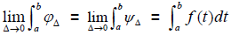is said to be integrable, where f(t) is the true probability density function and dt is an infinitesimally small true score interval width. The true score interval [a, b] can be extended to encompass the entire real line. The assumption that T is everywhere continuous ensures that all intervals over the real number line are integrable. By a similar argument, the probability density function f (e) can be constructed for the error random variable E.

The random variables T and E have expectations defined as 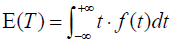and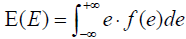, where t and e are points on the real number line. Given that real finite E(T) and E(E) exist, the variance of T and E can be defined as 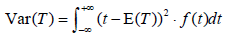and. The standard deviations for random variables T and E are defined as 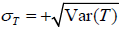and , under the assumption that finite positive variances exist.

Correlation between random variables T and E, however, requires analysis of joint outcome occurrences resulting from the conduct of a compound experiment. The outcomes of a compound experiment can be regarded as a set Ω_c of ordered pairs , where is the true construct amount andthe error amount assigned the i^th individual in the population. The set of ordered amount pairs can be equivalently represented as where is the Cartesian product defined as. Similarly, and .

Thus, the probability space for the compound experiment can be defined by the triplet . The probability function for the compound experiment can be constructed by first integrating over an interval of error scores Δ_E for a given true score and then integrating over the interval of true scores. The function is referred to as a joint probability density function and is denoted .

The covariance between random variables T and E is defined as . Given that Cov(T, E) exists, the correlation between T and E is. The requirement that Corr(T, E) = 0 requires that Cov(T, E) = 0, as σ_Tσ_E must be positive. The presence of true and error variation is a necessary condition in order for a causal relation to exist.

3. The true random variable T can be expressed as T = μ + λf, where μ = E(T), λ =σ_T , and f is the standardized true random variable. The classical true score equation can, by substitution, be expressed as X ≡ μ + λf + E. As standardization does not alter correlation, Corr(f, E) = 0 by assumption. The random variable f being a standardized variable has E(f) = 0 and Var(f) = 1. From this, it follows that E(X ) ≡ μ + λE(f) + E(E)= μ and Var(X) ≡ λ² Var(f) + Var(E) = λ² + Var(E).

As T is a random variable with assumed existent mean μ_T and finite standard deviation σ_T>0, the standardized true random variable f exists and is defined by . Consequently, it follows that T = μ_T +σ_T·f. This is equivalent to Raykov and Marcoulides Equation 4, where a_j = μ_T, b_j = σ_T , and T = f [21]. As f is a standardized variable, Var(f) = 1 by definition as opposed to by assertion as per the Raykov and Marcoulides formulation. Thus, the derived random variable X ≡ T + E can be equivalently expressed as X ≡ μ_T +σ_T·f + E, which is a single latent variable model. In that the standardized true random variable f is a latent variable, neo-classical test theory can be considered a latent variable measurement model. The converse does not necessarily follow. For an extended discussion of latent variable models, see [11].

4. Let X* be a standardized observed variable. Then X* ≡ λ/ (Var(X))^1/2f + E/(Var(X))^1/2; X* ≡ ( Var(T))^1/2/(Var(X))^1/2f + E*; X* ≡ (Var(T)/Var(X))^1/2f +E*; and X* ≡ (Var(T)/(Var(T) + Var(E)))^1/2f +E*. But Var(T)/((Var(T) + Var(E)) is defined as the reliability of X, denoted as ρ_XX in classical test score theory [1]. Therefore, X* ≡ λ*f + E*, where λ* = ρ^1/2_XX, referred to as the index of reliability. The implication is that reliability can be derived without reliance on the stipulation of equivalence of test-retest or parallel forms as in the classical theory.

By axiomatic assertion, an observed random variable X is defined as X ≡ T + E. From the algebra of expected values, it follows that E(X) ≡ E(T) + E(E) ≡ E(T) as E(E) = 0 by definition and Var(X) ≡ Var(T) + Var(E) + 2 Cov(T, E). From the premise that random variables T and E are uncorrelated, it follows that Cov(T, E) = 0, so that Var(X) ≡ Var(T) + Var(E) and . The standardized coefficient, where ρ_XX is the reliability of item X.

5. For the multivariate case of p observed items, define a p x 1 random vector X with elements X_i, i=1, 2, …, p, where X_i ≡ μ_i + λ_if_i + E_i. Suppose that all pairs fi and fj are perfectly correlated, i.e., Corr(f_i, f_j)=1. This is equivalent to requiring that f_i=f, i=1, 2, …, p, where f is referred to as a common standardized true random variable. The implication is that although the unstandardized true latent variable T_i may differ in location (expected value) and scale (standard deviation) across the p observed items contrary to the requirement of item equivalency in classical true-score theory, each observed item must assign an identical standardized true score to an individual subject.

The requirement that all observed items must manifest a common standardized true latent variable is the essence of the meaning of unidimensionality. Dimensionality refers to the number of constructs manifested by p items. If observed items are to be regarded as multivariate manifestations of a single construct, then it is imperative that all items assign the same standardized true score to a single subject, i.e., are unidimensional. Contrary to classical prescription, unidimensional observed items need not have equal true variance nor are they required to have equal error variance. All that is required is that item true scores be linearly related. The recognition that unstandardized item true scores need only be linearly related to maintain unidimensionality is credited to Phillip Rulon, and the condition referred to as essentially tau-equivalent [22,23]. Jöreskog termed models with a linear relation between true scores as congeneric [24]. Congeneric and essentially tau-equivalent models allow for any of the p unstandardized true random variables to serve as a comparative base. As a result, item loadings and true variance vary depending upon the base chosen. In contrast, designation of the standardized true variable as the common latent variable results in unit variance and item true standard deviations serving as item loadings, thereby allowing individual item reliabilities to be computed (see Tenet 4).

Linearly related true scores do not preclude the p items from varying in reliability. Those items with relatively high reliabilities can be regarded as markers of the true construct in that their observed variance is composed of a relative high proportion of true variance. Items can be ranked in order of quality according to their reliabilities computed as the square of their standardized latent variable loading.

It is easily shown that the presence of a common standardized true variable is sufficient to establish local independence. For all experimental subjects with a fixed standardized true score, f = k, as the only source of observed item variability is measurement error. But by assumption, error is uncorrelated across items and subjects. Thus, items are independent of each other for all subjects having equal common standardized true score, provided that the p item error variables are multivariate normally distributed. Furthermore, the unidimensional model with centered observed item variables meets the Rasch criterion of ratio invariance of items and experimental subjects. The conditional item expectation maintains a constant ratio for any two items over all subjects having equal score, as . Similarly, the ratio for any two subjects remains constant over all p items, as , which does not depend upon the item chosen.

6. Under the assumption that p latent unstandardized true variables T_i, i = 1, 2, …, p are perfectly correlated, the p x p population covariance matrix of observed items is : Σ = λλ` + ψ, where λ is a p x 1 vector of unstandardized true variable standard deviations and ψ is a p x p diagonal matrix of unstandardized error variances Var(E_i).

An element in the i^th row and j^th column of Σ is defined as . Substituting the posited true and error composition for each observed random variable gives . Simplifying and taking advantage of the distributive property of expected values allows the covariance to be expressed as . But and , as by definition, random error variables do not correlate with the common true score random variable nor with other random error variables. Thus, λλ` is a pseudo-covariance matrix of the p observed items. The term pseudo reflects that the diagonals contain only Var(T), whereas the off-diagonal entries are . The requirement that all true variables have nonzero finite variance ensures the presence of positive population item covariance. The error matrix ψ is diagonal to reflect the assumption that error random variables do not correlate with any other random variable except themselves. It is worth noting that all these model-implied structural relations hold only at the level of expected value due to defined error cancelation.

7. Designate x_α as a p x 1 vector of observed item scores for the α^th individual in a sample of size N randomly drawn from an infinite population. Assume that x_α ≡ μ + λf_α + ε_α, where μ is a p x 1 vector of item expected values, λ is a p x 1 vector of item latent coefficients, fα is an unobserved true score randomly drawn from a normal distribution with E(f) = 0 and Var(f) = 1, and ε_α is a p x 1 vector of unobserved error scores randomly drawn from a multivariate normal distribution with E(ε) = 0 and Cov(ε) = ψ. Furthermore, let all x_α be independently and identically distributed between as well as within individual subjects. This has the effect of ensuring that trial subpopulation distributions are identical to subject subpopulation distributions for a given item.

The random vector x_α is a specific instance of the vector X of random variables X_i, i = 1, 2, …, p, generally denoted by a lower case letter. The individual subject observed score model is a mixture of item and individual subject components, with individual components denoted by the subscript α. Each of the p items possesses an item mean and an item loading defined as the item true variable standard deviation. Each item assigns a fixed mean and loading to each individual sampled. Each sampled subject is randomly assigned a score on a common standardized true random variable as well as p measurement error scores.

Item and individual subject components are regarded to be independently determined. The experimental treatment process is assumed to be identical across subjects and replicated trials.

In order for a sample of size N to be considered as randomly drawn, not only must individuals be drawn from the same subject pool, but each draw must be independent of all other draws. Thus, replication across separate individuals in the experimental pool qualifies intuitively as a random sample. But replication by repeated draws of the same individual does not carry the same intuitive assurance. In order for the longitudinal draws to be considered as randomly drawn, each replication for a given subject is assumed to be independently sampled with replacement from the same population.

Independence across longitudinal within-subject replications is not a problem for error scores. The same cannot be said for individual true scores. Two conflicting true score interpretations are possible. One is that replications are each regarded as an independent random variable creating a within-subject time series over the replication domain. The requirement that item random variables at each time point be identically and independently distributed ensures that within-subject true scores fluctuate around a fixed item mean with common item variance. Time series with these characteristics are referred to as white noise. Then by the pointwise ergodic theorem, the between-subject true score distribution is identical to the within-subject distribution [25]. Between-subject distributional equivalence allows latent model parameters to be estimated cross-sectionally rather than longitudinally. The alternative interpretation as propounded by classical measurement theory is that individual true scores are fixed across replications, with only error scores allowed to vary. Statistically, this has the effect of treating individual true scores as incidental parameters, often referred to as nuisance parameters in that they cannot be independently estimated in the absence of a specified distributional form.

8. Let X and f have a joint multivariate normal distribution with mean vector (μ, 0)` and (p + 1) x ( p + 1) covariance matrix

.

The above consideration treats both the p observed item scores and the single standardized true variable f as random variables with means and covariance defined by existent expected values. The covariance between observed items and f is defined by the p x 1 vector λ, with entities being item true standard deviations. Covariance so defined satisfies Mill’s second condition for causality. Cross-sectional replication is equivalent to longitudinal replication. The measurement implication is that the causal process linking latent common true score to observed score is the same within individuals as between individuals. Constructs with this property are referred to as locally homogenous, where locally refers to the individual level of explanation and homogenous implies sameness across individual subjects [11].

9. The regression of the standardized common true variable f on X is E(f |X) = λ`( λλ` + ψ)^-1(x – μ) = (1 + Γ)^-1 λ` ψ<sup>-1</sup>(x – μ), where Γ = λ` ψ^-1λ. Consequently, the estimator of an individual common true score f_α is [26]. It should be noted that f_αμ is a Bayes estimator and that is a 1 x p v ector of unstandardized beta coefficients. Then the square of the multiple regression coefficient .

The squared multiple regression coefficient is termed R_Max and is equivalent to the squared canonical correlation between a weighted sum of p observed items and the standardized random true variable f [27]. Therefore, R_Max can be considered the maximum reliability that can be attained by an optimally weighted sum of p observed variables.

The regression true score estimator is Bayesian in that the estimate is conditional on knowing the observed score profile of an individual. The true score predictor provides a semantic connector between observed scores and the latent variable. If for all p items, then. In classical test theory, this is known as the Spearman-Brown prophecy formula. Thus, Spearman-Brown is but a special case of R_Max, where all items have equal reliabilities. The prophetic element follows from the use of multiple regression to predict the increase in R² resulting from the addition of equivalent item regressors. The origin of R_Max can be traced to Charles Spearman who derived the formulation as the maximum correlation between an optimally weighted sum of observed items and a common true score [28]. There is no reported evidence, however, that Spearman interpreted the multiple correlation in a maximum reliability context.

As R_Max is a squared multiple regression coefficient, the item with the highest reliability makes the greatest contribution to the reliability of the optimally weighted collection of items. Addition of items with lower reliabilities increases maximum reliability by decreasing increments. The decision as to whether to keep or delete items with lower reliability is at the researcher’s discretion.

10. The conditional expected value of the true score estimator is . Thus, f_α is an attenuated estimator of the latent standardized true score f_α An R_Max of near zero results in a true score estimate of near zero. Hence, the effect of lowered maximal reliability is regression toward the item mean. The attenuation, however, diminishes as R_Max→1. The mean square error in the estimate of the individual standardized true score f_α is [26]. As might be anticipated, maximization of the reliability of a weighed sum of observed items results in minimization of the mean square error in true score estimation and should be taken into consideration in the decision to drop or retain low reliability items.

Mean square error in the estimate of an individual true score is valid only in the context of true scores being defined as random rather than fixed effects. Consequently, true scores may vary across samples even though observed scores remain constant.

11. Common true score model parameters are estimated by confirmatory factor analysis using maximum likelihood estimation. All parameter estimates are consistent estimators and are designated by by. Parametric functions are estimated by replacing parameters with their sample estimates.

Maximum likelihood (ML) estimation renders unnecessary the core classical requirements of equivalent items and parallel forms. Instead, item true and error variances are uniquely estimated so as to minimize a ML fit function defined as , where log is the natural logarithm, λλ' +Ψ is the covariance structure generated by the common true score model, S is a sample item variance-covariance matrix, det is the determinant of a matrix, and trace is the sum of the main diagonal entries of a matrix [29]. All other parameters are as previously defined. Under the null hypothesis that S = λλ' +Ψ, f_ML = 0. As the disparity between observed sample and expected covariance structure increases, f_ML takes on ever larger positive values. Under the assumption that common true and error scores are multivariate normally distributed, (N – 1) f_ML is asymptotically distributed as chi square with p (p - 3)/2 dfs. Thus, rather than accept the common true score model as valid by definition, the null hypothesis of model fit can be empirically tested. Fit of the common true score model is considered empirical evidence that multiple items triangulate on the same construct and hence measure the same thing [30].

The fit function for testing the hypothesis of a common true score model can be equivalently expressed as , where all terms are as previously defined. The determinant of the sample covariance matrix, det(S), can be regarded as a generalized variance, thereby lending credence to the interpretation of det(S)(1 - R_Max) as a generalized coefficient of alienation. As the determinant of the error matrix det(ψ) deviates from that expected from the true score model, model fit becomes ever more problematic. The fact that R_Max can be equivalently expressed as , where is the standardized error variance for the i^th item, emphasizes that R_Max is maximized by minimization of item error variance and that model fit is a function of the interplay between minimized item error variance and the observed covariance matrix. If the null hypothesis of model fit is rejected, R_Max is not interpretable, as its meaning is derived from the premise of common true score unidimensionality.

Acceptance of the null hypothesis is empirical evidence for the existence of a common standardized true variable. If the null hypothesis is true, then (Σ −Ψ ) is of unitary rank and all second-order determinants must equal 0. As tetrads defined by Spearman as , where ρ_ij is an element in the i^th row and j^th column of the pseudo-correlation population matrix Σ* −Ψ* and and , are second order determinants, they must vanish, e.g., equal 0 under the condition that Σ* −Ψ* is of unitary rank [31]. A corollary is that the elements of Σ* −Ψ* are subject to the ratio equality , a condition denoted by Hart and Spearman and Spearman as internal consistency [32,33]. From this, one can conclude that the presence of a common true variable implies unitary rank and internal consistency. However, it does not follow that unitary rank necessarily implies a common true variable. If the null hypothesis of a common true variable is supported by the data, the implication is that the set of p observed items can be combined to create a test or a clinical scale, depending upon the nature of the constituent items. As all items can be assumed to measure an identical standardized latent true variable, item scores can be meaningfully combined into a weighted summated test or rating.

12. A distinction is drawn between statistical estimation and statistical prediction. Statistical estimation refers to the process of presently deriving parameter values based on observed sample scores. Statistical prediction refers to the use of point estimates to predict a score, usually based on an individual observed score profile not included in the original sample.

Maximum likelihood under the assumption of a multivariate joint distribution of p observed items and a single common true score affords a statistical method for estimation of minimized item error variances for a given sample. If the null hypothesis of unidimensionality is accepted, then a statistical estimation of individual true scores can be meaningfully derived using estimated model parameters. Under the assumption that a newly sampled individual not included in the original sample is drawn from the same multivariate population, the score profile of that individual can be used to predict what true score would have been assigned even though the individual was not in the original sample. The generative experiment is assumed to be comprised of a fixed set of p items potentially administrated to every subject in the population. This differs substantially from classical theory, which assumes that test items are drawn from a large domain set wherein all items are equivalent. Under classic test theory, this assumption is treated as an axiom and not subject to empirical test.

13. Both true score estimation and prediction are defined as. The distinction lies in the definition of the standard errors. If the true score estimator is a random effects model, the standard error of estimation of the mean standardized true score at is , where x_α is an individual score vector, X_C is a N x p matrix of sample centered observed individual score profiles, and is a sample estimate obtained by substituting estimated parameter values. The standard error of prediction of an individual common true score at is with all terms similarly defined with the exception of an added unity [34].

The estimated common true score is the conditional mean on the sample regression line for an observed score profile. The same value is used whether the true score is considered to be an estimate of the conditional mean or a prediction of an individual true score based on the observed score profile. The fact that only a conditional mean is estimated introduces an element of indeterminacy into true score estimation similar to that of factor indeterminacy [35]. A true score estimate can be constructed with a mean as a determinate part plus an indeterminate disturbance part. What differs between estimation and prediction is the interpretation of the standard error. The standard error of estimation is an estimate of the variability in the conditional mean expected to be introduced by repeated sampling from the experimental population. The standard error of prediction, in contrast, is an estimate of the variability in the prediction of an individual standardized true score based on an observed score profile across repeated sampling. As there is increased uncertainty introduced by prediction of an individual rather than a mean true score, the standard error of prediction is larger than the standard error of estimation. In both cases, the standard error is a function of estimated maximum reliability.

14. Confidence intervals are elliptical and increasing in width as the distance of the observed score profile from the mean profile becomes larger. The large-sample 95% confidence interval around the estimated mean true score is. The large-sample 95% confidence interval around a predicted true score for a given is and is larger than the confidence interval around the estimated conditional mean true score, as would be expected. The probability (1 – α) that the confidence interval contains the estimated or predicted value can be altered by appropriate choice of the (1 - α/2) point on the unit normal curve.

Both confidence intervals are the narrowest at the sample mean vector and fan out as the distances of the observed from the sample mean vector increases. The fan effect results from greater leverage being exerted by sample-induced variation in slope estimates at farther distances from the mean. Allowance for fanning confidence intervals circumvents one of the most damning criticisms of classic test theory.

Variable confidence intervals for future prediction of individual true scores are especially useful in psychopathological diagnosis and assessment where deviant scores are of special interest. Unlike the classical model, prediction error is greater for these individuals. The tradeoff is that more information is required regarding point estimates of model parameters. Computation of reliability from item correlations will no longer suffice. Covariance structure modeling needs to replace conventional dependency on simple covariance and correlation as intuitive measures. The effect will be to shift clinical emphasis from measurement of observables to statistical estimation of latent model parameters.

Neo-Classical Test Theory: Benefits and Costs

Neo-classical test theory as formalized by the fourteen tenets renders existent criticism of the classical model irrelevant. The test designation, while maintained, is expanded to include clinical scales and assessment instrumentation. The assumption of continuity moves the focus of testing from the certitudes of cognitive item correctness to the vicissitudes of cognitive thought [36]. Definition of random variables as functional transformations rather than empirical test scores provides an abstract connectivity between experimental outcomes and real numbers. Consideration of true and error random variables as primitives negates the claim that the theory is tautological. Utilization of theoretic concepts of measure theory allows random variable domains to be defined as probability spaces leading directly to the concept of continuous probability distributions and their use in the definitions of continuous variable means, variances, and covariance. The stipulation that individual observed and latent score profiles are independently and identically distributed across sample members eliminates the classical dependency on repeated observations on the same individual. Provision for testing the structural hypothesis of internal consistency nullifies Michell’s charge that classical test theory is pathological [14]. Regressing true scores on observed profile scores provides a random effects model for estimation of true score standard error of estimate. Separate estimation and prediction confidence bounds are computable and expand in width as the distance from the mean profile increases.

Reliability plays an ever more central role. Rather than test being axiomatically defined as in classical theory, unidimensionality of a collection of p fixed items is treated as a refutable hypothesis subject to empirical test. Fit of a common true-score model is a function of three sample statistics: the sample covariance matrix of the p items, the minimized estimate of item error variances, and an optimal reliability estimate. The optimal reliability, RMax, is defined as the square of the canonical correlation between the common true score and a weighted sum of the p fixed items. It is a known statistical fact that canonical correlation between a single variable and a weighted combination of p variables can be equivalently represented as a multiple regression equation with the single variable being regarded as the dependent variable, in this case the common true variable, and the p variables considered as regressors. The transition from correlation to regression allows item beta weights to be estimated, a multiple regression line determined, and fanning confidence bounds computed. The standard error of true scores is a function of R_Max and is a component of the standard errors of estimation and prediction. Unlike classical theory, there is always the lurking possibility that the set of p items may not admit to a unidimensional truescore structure. If so, then maximum reliability estimation is a meaningless exercise.

A longstanding controversy exists over the extent to which operations on real numbers must mirror operations on construct amounts. A specific point of contention is the charged failure of psychometricians to test the hypothesis that human attributes are quantifiable [14,37,38]. The argument is blunted by lack of differentiation between hypothesis as a testable proposition and axiom as a nontestable assertion. Neo-classical test theory as herein articulated ensures quantification by axiomatic assertion. Axioms as the building blocks of latent true score model construction cannot be falsified by direct empirical observation. Rather, axioms are ideations subject to the logical rules of consistency, completeness, and nonredundancy. The test of an axiomatic system is not correspondence of individual axioms with a descriptive representation of a native reality but the statistical fit of model-implied hypotheses with empirically obtained data. Model fit is a necessary but not sufficient condition. There is always the possibility that equivalent models fit the data equally as well or that alternative models may fit even better. The putative latent model is or should be the clinician’s best effort at constructing a micro worldview consistent with life experience, existent theories, and practical expediency. The goal of latent modeling is improved forecasting, prediction, and control over a felt but ultimately unknowable reality.

The downside is that structural modeling in the social and medical sciences is a more complex human activity requiring the building and testing of abstract micro-worlds. Unfortunately, operationalism and dependency on ANOVA with randomized sampling has led to declining awareness of and concern with measurement issues [39]. The rise in popularity of menu-driven statistical analysis programs has contributed to routinizing data analysis and its relegation to an appendant research task. Structural modeling, however, is steadily becoming an accepted data analytic procedure. Unfortunately, many of the same problems still persist, leading to research claims based on flawed analysis [40]. The entrenched predilection is to seek rejection of the null rather than fit of a proposed model. Connections between theoretical constructs and their representation in an abstract modeling world are often poorly articulated and the importance frequently ignored.

At root is lack of skills to navigate the world of the abstract. As Muthén has noted: “Presently, there is not enough done in the education of the ultimate users of these new statistical techniques for them to learn the methodological part of their research trade well” [40]. A recent survey by Aiken and colleagues confirms Muthén’s observation by reporting that “About half of graduate programs judged that few or none of their students were able to apply SEM” [41]. Lack of mathematical exposure is a major impediment. Whereas economists are conversant with calculus, most psychological researchers are not. Inclusion of mathematical topics in doctoral training is rare with the exception of mathematical psychology [41]. The armamentarium of mathematical topics needed to support sound measurement modeling includes set theory, functions and real numbers, matrix algebra, linear and characteristic equations, optimization theory as used in model estimation, continuous probability theory, and expected value algebra.

Not all users require the same degree of exposure. Muthén has identified three types: (i) those with substantive research interest for whom latent modeling is but another research methodology; (ii) those with an interest in latent modeling per se but do not envision contributing to the methodology; and (iii) those who aspire to contribute to methodological development [40]. The first group needs only knowledge of the existence and potential of latent variable modeling presented in a nonmathematical format. The second group requires knowledge about the procedures that move from modeling to statistical analysis. Knowledge about is gleaned from introductory math textbooks [42,43]; courses in quantitative methods, structural modeling, and applied statistics; topically relevant conferences and workshops; professional measurement journals and publications with a tutorial orientation; and the vast tutorial resources available on the Internet. The third group requires knowledge of how to develop models that advance the state-of-practice and is comprised primarily of advanced graduate and post-doctoral students with a Master’s degree in applied mathematics or applied statistics seeking substantive exposure to the social sciences.

Conclusion

The neo-classical latent measurement theory as herein articulated is offered as a modernization of classical test theory. Whereas classical theory is problematic, neo-classical theory embodies modern mathematical, statistical, and psychometric thinking and practice. Whereas the classical theory is oriented to a multiple-choice testing format, neo-classical theory is ideally suited for use with self-report questionnaires, scale construction, and clinical assessment. Whereas classical theory is weak, neo-classical theory is strong. But a strong measurement theory is no guarantee of strengthened research results. A generation of researchers conversant with abstract thinking and statistical modeling with latent variables is required. Hopefully, neo-classical test theory will serve as a catalyst for the improvement of measurement literacy.

References

1. Allen MJ, Yen WM (1979/2002) Introduction to measurement theory. Long Grove, IL: Waveland Press, Inc.
2. Eisenhart C (1983a) Laws of error I: Development of the concept. In Kotz S & Johnson NL (Edn), Encyclopedia of statistical sciences. Toronto: Wiley, 4: 530-547.
3. Eisenhart C (1983b) Laws of error II: The Gaussian distribution. In Kotz S & Johnson NL (Edn), Encyclopedia of statistical sciences. Toronto: Wiley, 4: 547-562.
4. Traub RE (1997) Classical test theory in historical perspective. Educ Meas Issues Pract 16: 8-14.
5. Kelley TL (1923) Statistical methods. New York: Macmillan.
6. Gulliksen H (1950) Theory of mental tests. New York: Wiley.
7. Novick MR (1966) The axioms and principal results of classical test theory. J Math Psychol 3: 1-18.
8. Lord FM, Novick MR (1968) Statistical theories of mental test scores. Reading, MA: Addison-Wesley.
9. Zimmerman DW (1975) Probability spaces, Hilbert spaces, and the axioms of test theory. Psychometrika 40: 395-412.
10. Zimmerman DW (2011) Sampling variability and the axioms of classical test theory. J Educ Behav Stat 36: 586-615.
11. Borsboom D (2005/2009) Measuring the mind. Cambridge, NY: Cambridge University Press.
12. Borsboom D, Mellenbergh GJ (2004) Why psychometrics is not pathological: a comment on Michell. Theory Psychol 14: 105–120.
13. Levy P (1969) Platonic true scores and rating scales: a case of uncorrelated definitions. Psychol Bull 71: 276-277.
14. Michell J (2000) Normal science, pathological science and psychometrics. Theory Psychol 10: 639-667.
15. Embretson SE (2004) The second century of ability testing: some predictions and speculations. Measurement 2: 1-32.
16. Borsboom D, Mellenbergh GJ, Van Heerden J (2003) The theoretical status of latent variables. Psychol Rev 110: 203-219.
17. Michell J, Ernst C (1996) The axioms of quantity and the theory of measurement. J Math Psychol 40: 235-252.
18. Michell J (1997) Quantitative science and the definition of measurement in psychology. Br J Educ Psychol 88: 355-383.
19. Sutcliffe JP (1965) A probability model for errors of classification. I: General considerations. Psychometrika 30: 73-96.
20. Cook TD, Campbell DT (1979) Quasi-experimentation: design & analysis issues for field settings. Chicago: Rand McNally.
21. Raykov T, Marcoulides GA (2016) On the relationship between classical test theory and item response theory: From one to the other and back. Educ Psychol Meas 76: 325-338.
22. lon PJ (1939) A simplified procedure for determining the reliability of a test by split-halves. Harv Educ Rev 9: 99-103.
23. Brennan RL (2011) Generalized theory and classical test theory. Appl Meas Educ 24: 1-21.
24. Jöreskog KG (1971) Statistical analysis of sets of congeneric tests. Psychometrika 36: 109-133.
25. Akcoglu MA (1966) Pointwise ergodic theorems. Trans Am Math Soc 125: 296-309.
26. Anderson TW (1984) An introduction to multivariate statistical analysis (2nd Edn). New York: Wiley.
27. Drewes DW (2000) Beyond the spearman-brown: a structural approach to maximal reliability. Psychol Methods 5: 214–227.
28. Bartholomew DJ, Deary IJ, Lawn M (2009) The origin of factor scores: Spearman, Thomson and Bartlett. B J Math Stat Psychol 62: 569-582.
29. Bollen KA (1989) Structural equations with latent variables. New York: Wiley.
30. Markus KA, Borsboom D (2011) The cat came back: evaluating arguments against psychological measurement. Theory Psychol 22: 452-466.
31. Spearman C (1904) General intelligence objectively determined and measured. Am J Psychol 15: 201-292.
32. Hart B, Spearman C (1913) General ability, its existence and nature. Br J Psychol 5: 51-84.
33. Spearman C (1914) The theory of two factors. Psychol Rev 21: 101-115.
34. https://www.sas.com/en_in/software/sas9.html
35. Schönemann PH, Wang M (1972) Some new results on factor indeterminacy. Psychometrika 37: 61-91.
36. Skinner BF (1989) The origins of cognitive thought. Am Psychol 44: 13-18.
37. Heene M (2013) Additive conjoint measurement and the resistance toward falsifiability in psychology. Front Psychol 4: 246.
38. Michell J (2004) Item response models, pathological science and the shape of error. Theory Psychol 14: 121-129.
39. Borsboom D (2006) The attack of the psychometricians. Psychometrika 71: 425-440.
40. Muthén BO (1989) Teaching students of educational psychology new sophisticated statistical techniques. In Wittrock MC & Farley F (Edn), The future of educational psychology. Hillsdale, NJ: Erlbaum Associates, pp: 181-189.
41. Aiken LS, West SG, Millsap RE (2008) Doctoral training in statistics, measurement, and methodology in psychology: replication and extension of Aiken, West, Sechrest, and Reno’s (1990) survey of PhD programs in North America. Am Psychol 63: 32-50.
42. Bishir JW, Drewes DW (1970) Mathematics in the behavioral and social sciences. New York: Harcourt, Brace and World.
43. Kaplan R, Kaplan E (2003/2014) The art of the infinite: the pleasure of mathematics. New York: Bloomsbury Press.