Keywords
Gold Atomic Clusters; Density-Functional Tight-Binding (DFTB)
approach; Finite-Differentiation Approximation; Force Constants (FCs); Normal
Modes of Vibrations
Introduction
Gold is an important material (resistant to most acids, used
in infrared shielding, colored-glass production, gold leafing,
and tooth restoration as well as a good conductor of heat and
electricity due to that it was attracted a great attention) and an
outstanding landmark in cluster science. Small clusters often
will have a different physical and chemical properties than their
bulk ones. Particularly, small particles of gold differ from the
bulk as they contain edge atoms that have low coordination and
can adopt binding geometries which lead to a more reactive
electronic structure [1,2].
The study of nanostructured materials exhibiting novel properties
is one of the most fascinating fields of current research. Small nanomaterials are of particular interest because of intriguing
characteristics [3-6]. Nanoparticles with smaller dimensions may
exhibit different properties in comparison with bulk material.
The nanoparticles possess unique physico-chemical, opticaland
biological properties which can be manipulated suitably for
desired applications [7]. Particulary, gold chemistry plays a very
important role in nanoelectronics and bionanosciences [8].
In the present work, we apply a parameterized density
functional tight-binding method combined with an numerical
differentiation-finite difference method on gold clusters with
from 3 to 20 atoms. We have extracted the normal modes of
vibration and the respective frequencies of the clusters, classified
according to their symmetry group. However, we only study on
the behaviour of the vibrational spectrum which are existed in
small neutral gold clusters at low-temperatures, T=0. In addition,
we provide computational evidence of the existence of the novel
properties of the interatomic interaction energy of the atoms
within the clusters.
Theoretical and Computational
Procedure
The DFTB9–11 is based on the density functional theory of
Hohenberg and Kohn in the formulation of Kohn and Sham. In
addition, the Kohn-Sham orbitals Ψi(r) of the system of interest
are expanded in terms of atom-centered basis functions
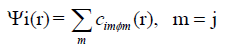 (1)
(1)
While so far the variational parameters have been the realspace
grid representations of the pseudo wave functions, it will now be
the set of coefficients cim. Index m describes the atom, where fm is centered and it is angular as well as radially dependant. The fm is determined by self-consistent DFT calculations on
isolated atoms using large Slater-type basis sets. In calculating
the orbital energies, we need the Hamilton matrix elements and
the overlap matrix elements. The above formula gives the secular
equations
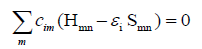 (2)
(2)
Here, cim’s are expansion coefficients, ei is for the single-particle
energies (or where ei are the Kohn-Sham eigenvalues of the
neutral), and the matrix elements of Hamiltonian Hmn and the
overlap matrix elements Smn are defined as
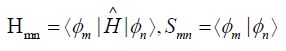 (3)
(3)
They depend on the atomic positions and on a well-guessed
density r(r). By solving the Kohn-Sham equations in an effective
one particle potential, the Hamiltonian ˆH is defined as
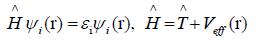 (4)
(4)
To calculate the Hamiltonian matrix, the effective potential
Veff has to be approximated. Here,  being the kinetic-energy
operator
being the kinetic-energy
operator 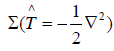 and Veff (r) being the effective Kohn-Sham
potential, which is approximated as a simple superposition of the
potentials of the neutral atoms,
and Veff (r) being the effective Kohn-Sham
potential, which is approximated as a simple superposition of the
potentials of the neutral atoms,
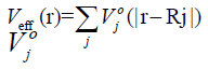 (5)
(5)
is the Kohn-Sham potential of a neutral atom, rj = r-Rj is an
atomic position, and Rj being the coordinates of the j-th atom.
The short-range interactions can be approximated by simple pair
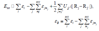
potentials, and the total energy of the compound of interest
relative to that of the isolated atoms is then written as,
 (6)
(6)
Here, the majority of the binding energy  is contained in the
difference between the single-particle energies Ɛi of the system
of interest and the single-particle energies
is contained in the
difference between the single-particle energies Ɛi of the system
of interest and the single-particle energies  of the isolated
atoms (atom index j, orbital index mj),
of the isolated
atoms (atom index j, orbital index mj),  is determined as
the difference between
is determined as
the difference between  and
and for diatomic molecules
(with being the total energy from parameter-free densityfunctional
calculations). In the present study, only the 5d and
6s electrons of the gold atoms are explicitly included, whereas
the rest are treated within a frozen-core approximation [9-12].
for diatomic molecules
(with being the total energy from parameter-free densityfunctional
calculations). In the present study, only the 5d and
6s electrons of the gold atoms are explicitly included, whereas
the rest are treated within a frozen-core approximation [9-12].
Structure of the Gold Atomic Clusters
Initially, a study on the structural and electronic properties of
the global minimum gold cluster structures was obtained by
combination of a genetic algorithm together with DFTB energy
calculations [13]. Dong and Springborg study explicitly includes the electronic degrees of freedom. This feature turned out to
be crucial since the electronic properties of the gold clusters
seem to play an important role in the determination of their
structure. When including orbital interactions, packing effects as
well as directional interactions determine the cluster structure.
Packing effects lead to high symmetry structures and to the
so-called magic numbers. Including orbital interactions in the
calculations leads to a partial suppression of the magic-numbers
and to low-symmetry structures. In most other metals, packing
effects are predominant. On the other hand, the structures of
most covalent molecules are determined by orbital interactions.
For gold clusters, both seem to be important. Springborg and
Dong suggest, that it is exactly this competition between packing
effects and directional interactions which leads to low-symmetry
clusters.
In their study, Dong and Springborg found the transition from
planar to three-dimensional structures for too small cluster sizes
N [14,15]. This could eventually be explained by the use of the
parametrized DFTB method. However, low-symmetry structures
have been found in other, more accurate studies on selected
cluster-sizes, too. The comparison of their results with results from
spherical-jellium-model calculations revealed some important
differences. The stability-function, which gives information about
particularly stable and unstable structures has much lower oddeven
amplitudes compared to the stability function obtained
within the jellium-calculations. This can be attributed to the
lower symmetry. The structures do not resemble to fragments
of crystalline gold-phases. Nevertheless, some regular patterns
are found, e.g. the clusters with size up to 20 atoms are built up
of atomic shells
Molecular Vibrations
In this section, we are going to introduce the mathematical
formalism on which the developed method is based. We will see
that, treating the problem within the so called normal-modeharmonicoscillator
(NMHO) approximation [16], the introduction
of the Hessian matrix and its diagonalization ultimately leads
to the eigenfrequencies of the system and its eigenvectors,
describing the harmonic motion of the clusters atoms [17].
Small vibrations in classical mechanics
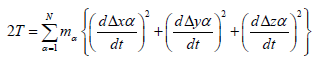
Let us consider a stable structure consisting of N atoms. Let xa;ya
and za be the coordinates of the ath atom of the structure and
aa;ba and ca the values of the equilibrium positions of the ath
atom. Displacements from the equilibrium positions can then be
expressed by Δxα = (xα-aα); Δyα = (yα-bα); Δzα = (zα-cα). In the above
notation, the classical kinetic energy T of the structure is given by
 (7)
(7)
It is customary to express the coordinates Δx1; :::; ΔzN by a new
set of so called mass weighted coordinates q1; :::;q3N, defined as
follows
 (8)
(8)
In terms of the time derivatives of these coordinates, the kinetic
energy is
 (9)
(9)
NMHO approximation and re-optimization
We start out with structures that have been optimized [13]. That
means that we have found the lowest total energy and that the
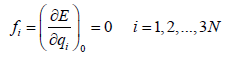
forces on the atoms are vanishing. We may then write the total
energy in a Taylor series around the optimized structure, so the
total energy depends on the positions of the atoms relative to each
other and therefore depends on the q’s. For small displacements,
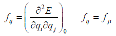
the total energy E may be approximated as a Taylor series in q,
within the actual normal-mode-harmonic-oscillator (NMHO)
approximation, the cubic and higher order terms are neglected
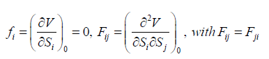
in the Taylor series, where the coefficients fi and fij are given by
 (10)
(10)
 (11)
(11)
This procedure implies a few customary consequences on which
the popularity of the NMHO-model is based. First of all, since
the energy has become quadratic, the vibrational motion we
get solving Newton’s equations of motion will be harmonic. The
further formulation of the problem leads to the Hessian matrix of
the system, which allows us a simple analysis of the vibrational
motion of the observed system. In the chosen notation, Newton’s
equation of motion can be cast in the form
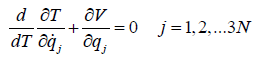 (12)
(12)
we get, the equation determining the motion of the coordinates
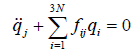 (13)
(13)
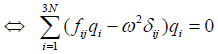
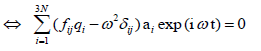
This is a set 3N simultaneous second-order linear differential
equations. A possible solution is  and
derivation with respect to time yields to
and
derivation with respect to time yields to  and can be
written as
and can be
written as
 (14)
(14)
 (15)
(15)
here, δij is called the Kronecker delta.
 (16)
(16)
 (17)
(17)
Dividing by 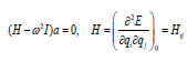 leads to a set of 3N algebraic
equations: Introducing matrix notation, we get
leads to a set of 3N algebraic
equations: Introducing matrix notation, we get
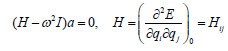 (18)
(18)
where  is the Hessian matrix containing the second
partial derivatives of the total energy of the system with respect
to the structure (mass-weighted) coordinates of the nuclei. E
being the total energy of the molecule/cluster, i.e. the single
point energy. I is the identity operation in
is the Hessian matrix containing the second
partial derivatives of the total energy of the system with respect
to the structure (mass-weighted) coordinates of the nuclei. E
being the total energy of the molecule/cluster, i.e. the single
point energy. I is the identity operation in  ,
, is a column vector containing the amplitudes ai
and the
is a column vector containing the amplitudes ai
and the  are the frequencies.
Equation (12) has non-vanishing solutions only, if
 (19)
(19)
Hence, the frequencies are obtained by consulting the roots of
the characteristic polynomial, i.e., the frequencies are obtained
by finding the eigenvalues of the Hessian matrix H.
In the case of a structure situated at a minimum on the
energy surface the Hessian matrix should be symmetricpositivesemidefinite
and therefore hermitian. It can be shown that
the eigenvectors of an hermitian matrix 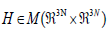 constitute
an orthonormal basis (onb) of
constitute
an orthonormal basis (onb) of  . The representation of the
Hessian matrix in this basis is diagonal and the diagonal elements
are the sought eigenfrequencies
. The representation of the
Hessian matrix in this basis is diagonal and the diagonal elements
are the sought eigenfrequencies 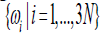
Moreover, the corresponding eigenvectors  of H are
the directions of the harmonic motions of the molecule. They
constitute the so-called normal modes. To fully specify any
N-atomic structure or its vibrational motion, only ((3N-5) for
linear and (3N-6) for non-linear) basis-vectors are needed. The
five/six remaining basis vectors span Kernel of the Hessian, i.e.,
they determine the absolute position and orientation of the
molecule in the inertial system. Thus, there are only ((3N-5) for
linear and (3N-6) for non-linear) linearly independent vibrations,
the molecule can undergo. From the construction of H, it follows
that the molecules motions along the normal modes are harmonic
oscillations. Moreover, since we are in a linear approximation,
every possible harmonic motion of the molecule can be written
as a linear combination of the normal modes.
of H are
the directions of the harmonic motions of the molecule. They
constitute the so-called normal modes. To fully specify any
N-atomic structure or its vibrational motion, only ((3N-5) for
linear and (3N-6) for non-linear) basis-vectors are needed. The
five/six remaining basis vectors span Kernel of the Hessian, i.e.,
they determine the absolute position and orientation of the
molecule in the inertial system. Thus, there are only ((3N-5) for
linear and (3N-6) for non-linear) linearly independent vibrations,
the molecule can undergo. From the construction of H, it follows
that the molecules motions along the normal modes are harmonic
oscillations. Moreover, since we are in a linear approximation,
every possible harmonic motion of the molecule can be written
as a linear combination of the normal modes.
The finding of the frequencies of the normal modes of the
clusters involves an eigenvalue problem which can be solved by
diagonalization of the symmetric positive semidefinite Hessian
matrix of the system. So, in the present study, two different
numerical diagonalization methods have been applied. The
first method bases on Jacobi-transformations of the symmetric
Hessian. The second method relies on the Househoulder-reduction
of the symmetric Hessian to a tridiagonal form and subsequent
application of a QLalgorithm which yields the eigenvalues and
vectors. Both methods are standard procedures and a complete
and comprehensive description is given in the Numerical Recipes,
both methods were implemented in the main-program unit
without any modifications with respect to the subroutine-codes
presented [18,19]. Within the numerical error, both methods
yield the same results.
The normal mode harmonic oscillator (NMHO)
approximation
Please note, that from now on, for convenience, the total energy
E of equation 6 in section 2 has the meaning as a potential
energy surface V. The potential energy depends on the positions
of the atoms relative to each other and therefore depends on
the q’s. For small displacements, the potential energy V may be
approximated as a Taylor series in q.
Now, we express the potential energy as a Taylor series.
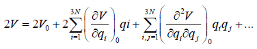 (20)
(20)
 (21)
(21)
and with
 (22)
(22)
W. l. o. g., V0 can be set to zero. And since the qi’s are the distances
from the equilibrium positions, the potential energy must have a
minimum at
{qi = 0 | i = 1,2,.., 3N}, (23)
and we get
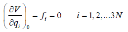 (24)
(24)
Within the actual normal-mode-harmonic-oscillator (NMHO)
approximation, the cubic and higher order terms are neglected
in the above series, such that the energy expression (19, 20)
becomes
 (25)
(25)
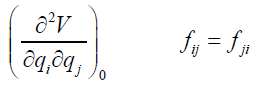
where the coefficients fij are given by
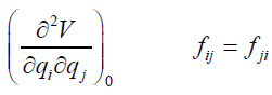 (26)
(26)
This procedure implies a few customary consequences on which
the popularity of the NMHO-model is based. First of all, since
the potential has become quadratic, the vibrational motion we
get solving Newton’s equations of motion will be harmonic. The
further formulation of the problem leads to the Hessian matrix of
the system, which allows us a simple analysis of the vibrational
motion of the observed system.
Numerical Differentiation: Finite
Difference Method
For the purpose of the present study, a very high accuracy
of the optimum structures is required. In a first approach,
we attempted to re-optimize the structures using the same
steepest-descent method which has already been used for the first optimization [13]. The vibrational properties are
treated within the normal-mode harmonic oscillator model
[16]. Therefore, we needed to find a suitable scheme to set up
the Hessian matrix of the system. Since we were using densityfunctional
tight binding energy calculations, we do not have
an analytical expression for the energy. Thus, we have to rely
on numerical differentiation. Subsequently, we had to test the
results in order to find suitable sets of differentiation parameters,
i.e., suitable combinations of differentiation step-size and order
of the polynomial. In order to get clusters which are somewhat
closer to the actual minimum on the potential energy surface,
we turned to a new strategy. This new strategy relies on the
properties of the Hessian eigenvectors. Based on the assumption,
that in the proximity to a minimum, the curvature of the potential
energy surface does only change very little, we developed a
method which could actually cope with the high numerical accuracy of the local structure optimization. Briefly, this method
is described as follows: The Hessian matrix is represented in an orthonormal basis consisting of the six
eigenvectors of the Hessian matrix which span its kernel and of
(3N-6) arbitrarily chosen mutually orthonormal basis vectors,
which are orthogonal to the kernel-eigenvectors. When
represented in this basis, the Hessian should be partially diagonal.
The diagonal part is now cut away and the remaining Hessian is
diagonalized to reveal the eigenfrequencies of the clusters normal
modes. Through the obtained eigenfrequencies, it is possible to
set up the vibrational partition function of the examined systems,
which gives access to the sought thermodynamic properties.
The Hessian matrix is the matrix of second derivatives of the
energy with respect to geometry which is quite sensitive to its
geometry. Energy second derivatives are evaluated numerically.
Themmass-weighted Hessian matrix is obtained by numerical
differentiation of the analytical first derivatives, calculated at
geometries obtained by incrementing in turn each of the 3N
nuclear coordinates by a small amount ds with respect to the
equilibrium geometry. The introduction of the Hessian matrix and
its diagonalization ultimately leads to the eigen-frequencies of the
system and its eigenvectors, describing the harmonic motion of
the clusters atoms. In order to obtain the matrix elements Hi j of
the Hessian matrix which are needed if one wishes to investigate
the clusters thermodynamic properties and one should obtain
the derivatives of potential energy surface (PES).
Cutting off the kernel
The Hessian matrix H is symmetric by Schwarz’ theorem. The
Kernel of H consists of all vectors which describe pure translational
and rotational motion of the center of mass of the molecule,
leaving its internal structure untouched. This is the eigenspace
of H which is associated to the eigenvalue 0. As we have 5 for
linear 6 for non-linear degrees of freedom corresponding to such
translations and rotations, dim(Ker(H)) = 5/6. We denote the five/
six Hessian eigenvectors associated to the Kernel  . The remaining (3N-5)/(3N-6) Hessian eigenvectors denoted
by
. The remaining (3N-5)/(3N-6) Hessian eigenvectors denoted
by 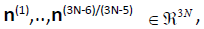 form a basis of the (3N-5)/(3N-6) dimensional configuration space, in which the molecular structure
may be described uniquely without any reference to the position
or orientation of the molecule relative to an inertial system. In
our new method, we apply the Gram-Schmidt theorem, to set up
an orthonormal basis for
form a basis of the (3N-5)/(3N-6) dimensional configuration space, in which the molecular structure
may be described uniquely without any reference to the position
or orientation of the molecule relative to an inertial system. In
our new method, we apply the Gram-Schmidt theorem, to set up
an orthonormal basis for  . The basis of the Kernel consisting
of the five/six hessian eigenvectors
. The basis of the Kernel consisting
of the five/six hessian eigenvectors  can easily be
found, they are the orthonormalized translations and rotations
of the structure. Now, we simply use as the first five/
six basis vectors for an orthonormal basis of denoted C. The
remaining (3N- 5)/(3N- 6) basis vectors of C are the arbitrarily
chosen mutually orthonormal vectors
can easily be
found, they are the orthonormalized translations and rotations
of the structure. Now, we simply use as the first five/
six basis vectors for an orthonormal basis of denoted C. The
remaining (3N- 5)/(3N- 6) basis vectors of C are the arbitrarily
chosen mutually orthonormal vectors  , which
have to satisfy
, which
have to satisfy  for any possible combination of i and j.
By construction, the basis vectors c(1),…,c(3N-5)/(3N-6) of basis C form a
basis of the (3N-5)/(3N-6) dimensional configuration space which
is the subspace of  configuration space, the normal
modes n do not contain any components of the basis of the kernel of the Hessian. Thus, the normal modes n satisfying the condition
configuration space, the normal
modes n do not contain any components of the basis of the kernel of the Hessian. Thus, the normal modes n satisfying the condition can be expanded
in the basis c(1),…,c(3N-5)/(3N-6) of the configuration space and they
will still be orthonormal. Now, let us represent H in the basis
C. Let
can be expanded
in the basis c(1),…,c(3N-5)/(3N-6) of the configuration space and they
will still be orthonormal. Now, let us represent H in the basis
C. Let  be the matrix consisting of the column
vectors of C, i.e.,
be the matrix consisting of the column
vectors of C, i.e.,
 (27)
(27)
Since U is a unitary transformation, the complex-conjugate of U is
equal to its inverse, i.e., U* =U-1 and thus the sought representation H’ of H in the new basis C is found by calculating U*HU = H’ Since the first five/six vectors basis of the basis C are
the eigenvectors corresponding to translation and rotation, the
first five/six lines and columns of the representation H’ of H in this
basis should be diagonal and the eigenvalues which are the H' ’s
diagonal elements should be equal to 0.
Diagonalization of the non-diagonal submatrix H’’ Ɛ which is the representation of the
Hessian in the basis c(1),…,c(3N-5)/(3N-6) of the configuration space,
yields its eigenvectors, i.e., the (3N-5)/(3N-6) normal modes
which is the representation of the
Hessian in the basis c(1),…,c(3N-5)/(3N-6) of the configuration space,
yields its eigenvectors, i.e., the (3N-5)/(3N-6) normal modes  The diagonal elements are
the sought eigenvalues, the eigenfrequencies of the normal
modes which are needed for the calculation of thermodynamic
properties.
The diagonal elements are
the sought eigenvalues, the eigenfrequencies of the normal
modes which are needed for the calculation of thermodynamic
properties.
First, we set up an orthonormal basis which allows to separate  into its (3N-5)/(3N-6)-dimensional configuration subspace and
the complementary five/six dimensional subspace which makes
reference to absolute position and orientation of the molecule.
The latter is not needed for the description of the molecule’s
structure and the normal modes. Second, we represent the Hessian in this basis and cut away the part belonging to the five/
six-dimensional complementary space, before the new Hessian
into its (3N-5)/(3N-6)-dimensional configuration subspace and
the complementary five/six dimensional subspace which makes
reference to absolute position and orientation of the molecule.
The latter is not needed for the description of the molecule’s
structure and the normal modes. Second, we represent the Hessian in this basis and cut away the part belonging to the five/
six-dimensional complementary space, before the new Hessian  finally is diagonalized to
reveal its eigenvalues and vectors. For quite all systems, results
obtained in both ways, with the above method and without it
were compared. The results are very close to each other. The
numerically optimized structures are almost exact and/or the
Hessian matrix changes very little around the minimum and the
numerical error can be ignored, using an appropriate method.
Applying the new method in our further calculations, we were
able to find positive semi definite Hessian matrices H’’ for all
structures.
finally is diagonalized to
reveal its eigenvalues and vectors. For quite all systems, results
obtained in both ways, with the above method and without it
were compared. The results are very close to each other. The
numerically optimized structures are almost exact and/or the
Hessian matrix changes very little around the minimum and the
numerical error can be ignored, using an appropriate method.
Applying the new method in our further calculations, we were
able to find positive semi definite Hessian matrices H’’ for all
structures.
Calculation of numerical force constants (fcs) and
vibrational frequency
A re-optimized structure of the force constants (FCs) could
be extracted from the already optimized structure [13] as the
following, the force(s) expressions were obtained by derivation
of the energy expression (or) from the expression of energy, the
forces can be easily calculated by derivation. Here, the Force(s) Fj that act on the j-th atom of the system can be calculated applying
the Hellmann-Feynman theorem [20,21], so the forces are given as
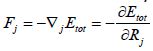 (28)
(28)
These are all identical to 0 (within numerical accuracy) for the
optimized structure [13]. Interatomic forces can easily be derived
from an exact calculation of the gradients of the total energy at
the considered atoms site, finally, the forces acting on an atom at
Rj are obtained as follows:
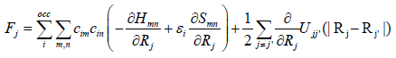 (29)
(29)
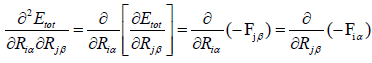
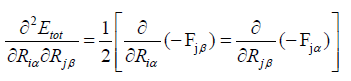
In our case, we have calculated as the numerical first-order
derivatives of the forces instead of the numerical-second-order
derivatives of the total energy. In principle there is no difference,
but numerically the approach of using the forces is more accurate
and, moreover, it requires much less calculation. However, to
extract the force constants (FCs) in a atomic cluster directly,
rather than indirectly through the agency of energy, a finite
difference formula has been introduced as following.
We obtained our results by using the following formula,
 (30)
(30)
 (31)
(31)
So for convenience eqn. (30 and 31) can be written as,
 (32)
(32)
 (33)
(33)
for homonuclear case, M represents the atomic mass,
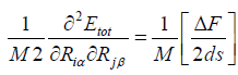 (34)
(34)
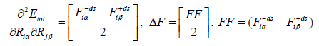
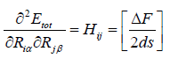
When the forces on atoms are known, the FCs can be used to
compute relaxations and relaxation energies. In total we end
up with (3N×3N) values  . The complete list of these force
constants (FCs) is called the Hessian Hi j, which is a (3N _3N)
matrix. Here, i is the component of (x, y or z) of the force on
the j’th atom, so we get 3N. DF is the average difference of the
two first derivatives of the force constants (FCs) and ds is a small
displacement within the nuclear coordinates. We found that a
PES over which the gradients extend for a small displacements
ds = ±[0:01] a.u. of equilibrium coordinate value of cluster,
which is a reasonable value and allowed to discriminate between
the translational, rotational motion (Zeroeigenvalues) and the
vibrational motion [ i is vibrational frequencies [(low(min),
high(max))] (Non-Zero-eigenvalues) of the atoms (or molecules)
of the Hessian eigenvalues.
. The complete list of these force
constants (FCs) is called the Hessian Hi j, which is a (3N _3N)
matrix. Here, i is the component of (x, y or z) of the force on
the j’th atom, so we get 3N. DF is the average difference of the
two first derivatives of the force constants (FCs) and ds is a small
displacement within the nuclear coordinates. We found that a
PES over which the gradients extend for a small displacements
ds = ±[0:01] a.u. of equilibrium coordinate value of cluster,
which is a reasonable value and allowed to discriminate between
the translational, rotational motion (Zeroeigenvalues) and the
vibrational motion [ i is vibrational frequencies [(low(min),
high(max))] (Non-Zero-eigenvalues) of the atoms (or molecules)
of the Hessian eigenvalues.
The vibrational partition function
The vibrational partition function is calculated by normal mode
analysis. The partition function yields all equilibrium thermal
properties of the clusters and harmonic approximation was used
in the calculation of the vibrational contribution to the cluster
partition function. Reducing dimensionality can bring entirely
new properties for the thermodynamics of vibrational states for
nanoclusters. The one-dimensional vibrational partition function
zvib expressed by a sum over all possible vibrational states of the
system,
 (35)
(35)
kB is Boltzmann’s constant, T is the absolute temperature
and Ei is the energy corresponding to the vibrational state
i. Each vibrational state of the system consisting of (3N-5)/
(3N-6) harmonic oscillators which are by construction linearly
independent. The partition function of a cluster is evaluated in
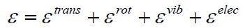
the same way one would evaluate that of a polyatomic molecule.
The energy of cluster or molecule is assumed to be separable
[22], i.e.,
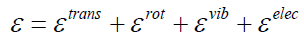 (36)
(36)
will influence each other. For example, eqn. (35) implies that the
curvature of the potential energy surface of the electronically
excited molecule is the same as for the molecule in its electronic
ground state. This is a necessary condition for the vibrational
frequencies and therefore for the vibrational energy to be
independent from the electronic state of the molecule. Also, if
the energy surfaces of the ground state and an electronically
excited state come close together (avoided crossing), the
separability of the electronic and vibrational modes may be
a poor approximation (breakdown of the Born-Oppenheimer
approximation) [22]. Similarly, rotational excitation will have an
impact on the bond length of "floppy" (soft bending potential)
molecules and subsequently on the vibrational levels [22].
However, it can be shown that, for sufficiently low temperatures, the coupling effects are small and can be neglected, because
the molecule is not likely to be in a highly excited state, where
coupling becomes important. As long as the vibrations can be
treated within the harmonic-oscillator-normal-mode model,
the anharmonicity of the potential can be neglected and the
average bond lengths won’t increase with vibrational excitation.
Under the assumptions implied by eqn. (35), we can re-write the
molecular partition function in a factorized form,
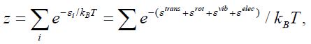 (37)
(37)
where the sum has to be performed over all combinations of
vibrational, rotational, translational and electronic states
 (38)
(38)
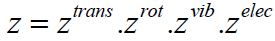
But the above result is just the product of partition functions
which only take into account a single mode of excitation, i.e.,
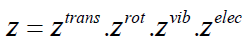 (39)
(39)
This result shows that in the case of negligible coupling of the
different excitations it is possible to approximate the partition
function as a product of translational, rotational, vibrational and
electronic partition functions.
The individual contributions
In the present work, we focus on the size and temperature
dependence of the vibrational part of the heat capacity. It was
demonstrated, that the approximations introduced by the
harmonicoscillator-normal-mode model, which imply that the
different vibrational modes can be treated independently from
each other, lead to a factorization of the vibrational partition
function itself. This work does not answer the question, whether
the electrons are irrelevant for the thermodynamic quantities
or not. Most often, the electronic excitation energies are much
larger than Kt and we are going to neglect the electronic partition
function. We still need to find expressions for the translational,
the rotational and the vibrational partition functions, so as to get
access to the partition function and subsequently to the heat
capacity we seek. According to the above and to eqn. (38), as an
enabling the cluster partition function to be written as a product
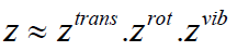 (40)
(40)
In the literature, approximate formulae for the translational and
the rotational part of the partition function are derived [23]. The
translational part ztrans is related to center of mass translation
and can approximatively be treated within the ideal-gas model.
An approximate formula for the rotational part zrot is found by
application of the concepts of a rigid rotator on the cluster’s
structure. However, based on the equipartition theorem in
classical statistical thermodynamics, we know that in the case of
the classical limit, the internal energy of a system will distribute
itself evenly among its quadratic degrees of freedom if not only the
lowest corresponding energy levels are significantly populated,
but also the higher ones. The population of the quantum states
of a given degree of freedom is temperature dependent. The
closer the energies of the different quantum states lie together, the more probable it is to find a molecule in an excited state and
the lower will be the temperature for which the classical limit
is reached and the results of the equipartition theorem can
be applied. It can easily be shown that the energy differences
between the rotational and the translational states of a typical
system are small compared to kT [24-32]. The equipartition
theorem states, that each degree of freedom receives an
average energy of 1/2kT. Since translation and rotation (of a
nonlinear molecule) correspond to six degrees of freedom,
the contribution to the internal energy is 3kT. In the present
application, the translational and the rotational contributions
are treated according to the theorem described above and only
the vibrational partition function will be considered rigorously.
In the case of the classical limit, the rotational and translational
parts of the partition function do not depend on the cluster
structure. Since the (3N-6) oscillators are by construction linearly
independent, the vibrational energy can be expressed as a sum
of the vibrational energies of each independent mode, i.e.,
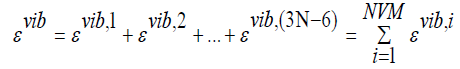 (41)
(41)
NVM being the number of normal vibrational modes of the
cluster. The vibrational partition function Zvib expressed by a sum
over all possible vibrational states of the system,
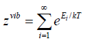 (42)
(42)
Ei is the energy corresponding to the vibrational state i. Each
vibrational state of the system consisting of (3N-6) harmonic
oscillators is defined by a distinct set {nj | j = 1,2,…,(3N-6)} of (3N-
6) vibrational quantum numbers,
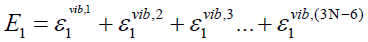 (43)
(43)
 (44)
(44)
 (45)
(45)
harmonic oscillator and the lower index specifies the quantum
state it is in. For our understanding, we can write
 (46)
(46)
And again, rearranging the terms in the above equation yields
a factorized vibrational partition function, i.e., a product of the
(3N-6) partition functions each of which describes one individual
harmonic oscillator,
 (47)
(47)
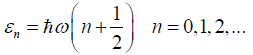
Recalling the energy states of the harmonic oscillator
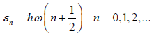 (48)
(48)
we are now in the position to give a concrete expression for the
vibrational partition function. Given ωi, the angular frequency of the i-th harmonic oscillator, the partition function describing it is
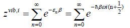 (49)
(49)
where we introduced the inverse temperature ß=1/kT.
Rearranging (48) leads us to
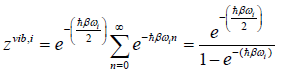 (50)
(50)
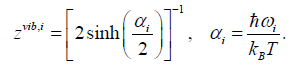 (51)
(51)
The contributions of translation and rotation depend only on the
mass and moment of inertia of the molecule, and they are thus
easy to calculate using the simple models of the particle in a box
and the rigid rotator, respectively. In contrast, the vibrational
contributions are, in general, difficult to evaluate, and thus are
the prime issue of this work. The individual terms in the product
are evaluated from standard statistical mechanical formulas
(using the harmonic approximation) to evaluate the vibrational
component zvib, Combining the above result with (46), we finally
see, that
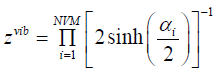 (52)
(52)
NVM is the number of normal vibrational modes of the cluster.
The above calculations were used to examine the helmholtz free
energy of formation of the clusters as a function of temperature.
Results and Discussion
In this article, we present only about the symmetric structure
of the gold atomic neutral clusters (Au3-20) and its vibrational
spectrum. The predicted spectrum ranges were found to be in
a range of 0.55 to 370.72 cm-1. By using a parameterized tightbinding
density-functional method combined with numerical
finite difference method we have confirmed the global total
energy-minimum structures for gold clusters containing up to
20 atoms. The calculated vibrational frequency ranges were
tabulated (Tables 1-18). Interestingly, we have observed some
double and triple state degeneracy at T= 0. In fact, Au6-8 clusters
are unique among the other clusters, due to their degeneracy
nature. Thus as a different molecule with atomic packing could
be similar to that of bulk gold but with very different properties
that is with respect to the electron density between the different
concentric layers. However, non-degenerate modes, because of
their higher symmetry, are easier to visualize at the spectrum. Interestingly, the lower non-degenerate mode displaces atoms
only at the edges, not at the vertices or face centers. Since
different symmetry gives rise to a large number of degenerate
modes, but only some distinct modes frequencies are expected
for the rest of the clusters. Furthermore, normal modes of
vibration are having both infrared and Raman-active, and the
remains are optically silent (which will have some experimental difficulties). Nevertheless, all interactions may be accompanied
by electron transfer and the interactions onto the vertex, edge,
or inner gold atoms. Density Functional calculations predict
that Au3-20 possesses a different geometry structures which
were then verified through the Gabedit package [25] (Tolerance
for principal axis classification: 0.00500 in angstrom (Å) and
Precision for atom position: 0.09399 in angstrom (Å)). In addition to that the predicted minima of the global structure optimization
of Au3 to Au20 were plotted in Figures 1-6 by increasing cluster
size and energy at T = 0 K. Overall, cluster size, spectrum ranges and the symmetry of gold clusters from N=3 to 20 atoms are also
mentioned at the Table 19.
Normal Vibrational
Modes (NVM=3) |
Vibrational frequency (ωi) in cm1 |
| 1 |
19.21 |
| 2 |
87.47 |
| 3 |
246.21 |
Table 1: Calculated vibrational frequency (ωi) of the re-optimized gold
cluster, Au3 at T=0.
| Normal Vibrational Modes (NVM=6) |
Vibrational frequency (ωi) in cm1 |
| 1 |
9.83 |
| 2 |
31.63 |
| 3 |
55.2 |
| 4 |
98 |
| 5 |
147.12 |
| 6 |
165.46 |
Table 2: Calculated vibrational frequency (ωi) of the re-optimized gold
cluster, Au4 at T=0.
| Normal Vibrational Modes (NVM=9) |
Vibrational frequency (ωi) in cm1 |
| 1 |
0.55 |
| 2 |
2.5 |
| 3 |
43.25 |
| 4 |
47.7 |
| 5 |
81.82 |
| 6 |
132.74 |
| 7 |
196.33 |
| 8 |
224.53 |
| 9 |
276.83 |
Table 3: Calculated vibrational frequency (ωi) of the re-optimized gold
cluster, Au5 at T=0.
| Normal Vibrational Modes (NVM=12) |
Vibrational frequency (ωi) in cm 1 |
| 1 |
2.44 |
| 2 |
2.44 |
| 3 |
2.44 |
| 4 |
38.59 |
| 5 |
38.59 |
| 6 |
58.51 |
| 7 |
58.51 |
| 8 |
118.06 |
| 9 |
164.08 |
| 10 |
178.3 |
| 11 |
282.99 |
| 12 |
282.99 |
Table 4: Calculated vibrational frequency (ωi) of the re-optimized gold
cluster, Au6 at T=0.
| Normal Vibrational Modes (NVM=15) |
Vibrational frequency (ωi) in cm1 |
| 1 |
20.48 |
| 2 |
20.48 |
| 3 |
40.78 |
| 4 |
55.5 |
| 5 |
55.5 |
| 6 |
58.63 |
| 7 |
58.63 |
| 8 |
106.38 |
| 9 |
106.38 |
| 10 |
109.62 |
| 11 |
142.05 |
| 12 |
142.05 |
| 13 |
214.62 |
| 14 |
214.62 |
| 15 |
235.19 |
Table 5: Calculated vibrational frequency (ωi) of the re-optimized gold
cluster, Au7 at T=0.
| Normal Vibrational Modes (NVM=18) |
Vibrational frequency (ωi) in cm1 |
| 1 |
4.66 |
| 2 |
4.67 |
| 3 |
24.52 |
| 4 |
24.53 |
| 5 |
24.53 |
| 6 |
64.97 |
| 7 |
67.92 |
| 8 |
67.92 |
| 9 |
67.92 |
| 10 |
102.72 |
| 11 |
102.72 |
| 12 |
102.72 |
| 13 |
131.45 |
| 14 |
131.45 |
| 15 |
198.97 |
| 16 |
215.07 |
| 17 |
215.08 |
| 18 |
215.08 |
Table 6: Calculated vibrational frequency (ωi) of the re-optimized gold cluster, Au8 at T=0.
| Normal Vibrational Modes (NVM=21) |
Vibrational frequency (ωi) in cm1 |
| 1 |
2.76 |
| 2 |
8.29 |
| 3 |
10.32 |
| 4 |
43.42 |
| 5 |
48.78 |
| 6 |
59.99 |
| 7 |
64.54 |
| 8 |
73.24 |
| 9 |
92.68 |
| 10 |
99.4 |
| 11 |
102.32 |
| 12 |
119.75 |
| 13 |
133.5 |
| 14 |
137.53 |
| 15 |
168.78 |
| 16 |
171.32 |
| 17 |
173.67 |
| 18 |
181.97 |
| 19 |
204.4 |
| 20 |
220.93 |
| 21 |
313.24 |
Table 7: Calculated vibrational frequency (ωi) of the re-optimized gold
cluster, Au9 at T=0.
| Normal Vibrational Modes (NVM=24) |
Vibrational frequency (ωi) in cm1 |
| 1 |
34.18 |
| 2 |
35.73 |
| 3 |
40.94 |
| 4 |
42.96 |
| 5 |
47.34 |
| 6 |
53.51 |
| 7 |
54.63 |
| 8 |
56.61 |
| 9 |
73.12 |
| 10 |
117.24 |
| 11 |
119.14 |
| 12 |
131.3 |
| 13 |
135.27 |
| 14 |
137.72 |
| 15 |
141.02 |
| 16 |
158.26 |
| 17 |
162.84 |
| 18 |
197.3 |
| 19 |
201.95 |
| 20 |
208.66 |
| 21 |
211 |
| 22 |
219.66 |
| 23 |
225.22 |
| 24 |
341.88 |
Table 8: Calculated vibrational frequency (ωi) of the re-optimized gold
cluster, Au10 at T=0.
| Normal Vibrational Modes (NVM=27) |
Vibrational frequency (ωi) in cm1 |
| 1 |
7.32 |
| 2 |
13.99 |
| 3 |
23.32 |
| 4 |
25.54 |
| 5 |
26.82 |
| 6 |
31.14 |
| 7 |
38.99 |
| 8 |
40.47 |
| 9 |
47.89 |
| 10 |
50.7 |
| 11 |
58.37 |
| 12 |
77.1 |
| 13 |
89.59 |
| 14 |
99.44 |
| 15 |
105.82 |
| 16 |
116.72 |
| 17 |
139.15 |
| 18 |
140.83 |
| 19 |
155 |
| 20 |
167.69 |
| 21 |
183.43 |
| 22 |
205.44 |
| 23 |
216.68 |
| 24 |
225.77 |
| 25 |
263.82 |
| 26 |
272.52 |
| 27 |
291.85 |
Table 9: Calculated vibrational frequency (ωi) of the re-optimized gold
cluster, Au11 at T=0.
| Normal Vibrational Modes (NVM=30) |
Vibrational frequency (ωi) in cm1 |
| 1 |
1.01 |
| 2 |
12.39 |
| 3 |
15.81 |
| 4 |
19.28 |
| 5 |
25.17 |
| 6 |
25.55 |
| 7 |
29.87 |
| 8 |
31.54 |
| 9 |
33.8 |
| 10 |
39.88 |
| 11 |
42.25 |
| 12 |
54.2 |
| 13 |
67.07 |
| 14 |
82.31 |
| 15 |
83.87 |
| 16 |
100.68 |
| 17 |
104.66 |
| 18 |
117.65 |
| 19 |
127.19 |
| 20 |
138.92 |
| 21 |
149.36 |
| 22 |
153.11 |
| 23 |
172.5 |
| 24 |
182.26 |
| 25 |
187.53 |
| 26 |
205.84 |
| 27 |
233.56 |
| 28 |
245.6 |
| 29 |
264.76 |
| 30 |
325.89 |
Table 10: Calculated vibrational frequency (ωi) of the re-optimized gold
cluster, Au12 at T=0.
| Normal Vibrational Modes (NVM=33) |
Vibrational frequency (ωi) in cm1 |
| 1 |
11.45 |
| 2 |
13.66 |
| 3 |
14.02 |
| 4 |
20.81 |
| 5 |
25.53 |
| 6 |
26.48 |
| 7 |
28.3 |
| 8 |
32.12 |
| 9 |
32.79 |
| 10 |
34.11 |
| 11 |
37.69 |
| 12 |
41.07 |
| 13 |
53.72 |
| 14 |
56.3 |
| 15 |
65.49 |
| 16 |
69.53 |
| 17 |
84.35 |
| 18 |
94 |
| 19 |
100.49 |
| 20 |
117.37 |
| 21 |
128.98 |
| 22 |
134.62 |
| 23 |
145.48 |
| 24 |
147.39 |
| 25 |
172.04 |
| 26 |
185.62 |
| 27 |
200.02 |
| 28 |
210.07 |
| 29 |
214.17 |
| 30 |
225.57 |
| 31 |
242.58 |
| 32 |
263.26 |
| 33 |
334.7 |
Table 11: Calculated vibrational frequency (ωi) of the re-optimized gold cluster, Au13 at T=0.
| Normal Vibrational Modes (NVM=36) |
Vibrational frequency (ωi) in cm1 |
| 1 |
17.02 |
| 2 |
18.86 |
| 3 |
19.53 |
| 4 |
19.75 |
| 5 |
24.31 |
| 6 |
25.34 |
| 7 |
27.18 |
| 8 |
34.04 |
| 9 |
34.53 |
| 10 |
38.67 |
| 11 |
42.79 |
| 12 |
43.21 |
| 13 |
44.63 |
| 14 |
58.46 |
| 15 |
58.89 |
| 16 |
69.39 |
| 17 |
70.86 |
| 18 |
84.22 |
| 19 |
84.87 |
| 20 |
92.74 |
| 21 |
109.7 |
| 22 |
113.59 |
| 23 |
130.96 |
| 24 |
132.76 |
| 25 |
147.38 |
| 26 |
152.9 |
| 27 |
167.18 |
| 28 |
176.74 |
| 29 |
181.82 |
| 30 |
182.93 |
| 31 |
186.81 |
| 32 |
198.47 |
| 33 |
203.39 |
| 34 |
215.87 |
| 35 |
225.76 |
| 36 |
240.2 |
Table 12: Calculated vibrational frequency (ωi) of the re-optimized gold
cluster, Au14 at T=0.
| Normal Vibrational Modes (NVM=39) |
Vibrational frequency (ωi) in cm1 |
| 1 |
7.49 |
| 2 |
12.27 |
| 3 |
17.09 |
| 4 |
22.53 |
| 5 |
23.59 |
| 6 |
31.08 |
| 7 |
34.1 |
| 8 |
42.3 |
| 9 |
47.22 |
| 10 |
48.84 |
| 11 |
60.25 |
| 12 |
67.56 |
| 13 |
69.45 |
| 14 |
73.36 |
| 15 |
74.69 |
| 16 |
80.68 |
| 17 |
90.49 |
| 18 |
92.83 |
| 19 |
96.03 |
| 20 |
102.7 |
| 21 |
106.87 |
| 22 |
112.73 |
| 23 |
119.17 |
| 24 |
136.82 |
| 25 |
137.6 |
| 26 |
148.91 |
| 27 |
151.87 |
| 28 |
162.23 |
| 29 |
168.74 |
| 30 |
177.56 |
| 31 |
190.79 |
| 32 |
200.3 |
| 33 |
202.73 |
| 34 |
207.81 |
| 35 |
218.03 |
| 36 |
231.37 |
| 37 |
238.11 |
| 38 |
282.44 |
| 39 |
285.36 |
Table 13: Calculated vibrational frequency (ωi) of the re-optimized gold
cluster, Au15 at T=0.
| Normal Vibrational Modes (NVM=42) |
Vibrational frequency (ωi) in cm1 |
| 1 |
17.13 |
| 2 |
21.26 |
| 3 |
22.19 |
| 4 |
30.59 |
| 5 |
31.41 |
| 6 |
36.5 |
| 7 |
40.37 |
| 8 |
43.02 |
| 9 |
46.15 |
| 10 |
49.37 |
| 11 |
56.35 |
| 12 |
57.66 |
| 13 |
58.24 |
| 14 |
66.67 |
| 15 |
75.28 |
| 16 |
77.28 |
| 17 |
83.12 |
| 18 |
85.97 |
| 19 |
89.07 |
| 20 |
99.59 |
| 21 |
110.56 |
| 22 |
116.51 |
| 23 |
120.99 |
| 24 |
131.27 |
| 25 |
142.26 |
| 26 |
155.39 |
| 27 |
155.74 |
| 28 |
180.46 |
| 29 |
183.1 |
| 30 |
185.17 |
| 31 |
190.34 |
| 32 |
192.71 |
| 33 |
204.67 |
| 34 |
215.89 |
| 35 |
219.11 |
| 36 |
233.45 |
| 37 |
252.64 |
| 38 |
261.57 |
| 39 |
269.35 |
| 40 |
272.28 |
| 41 |
285.58 |
| 42 |
295.76 |
Table 14: Calculated vibrational frequency (ωi) of the re-optimized gold
cluster, Au16 at T=0.
| Normal Vibrational Modes (NVM=45) |
Vibrational frequency (ωi) in cm1 |
| 1 |
9.57 |
| 2 |
10.23 |
| 3 |
11.81 |
| 4 |
12.98 |
| 5 |
16.73 |
| 6 |
18.47 |
| 7 |
20.67 |
| 8 |
21.59 |
| 9 |
24.78 |
| 10 |
26.02 |
| 11 |
26.95 |
| 12 |
31.39 |
| 13 |
32.96 |
| 14 |
38.97 |
| 15 |
45.72 |
| 16 |
50.75 |
| 17 |
58.65 |
| 18 |
59.62 |
| 19 |
62.98 |
| 20 |
65.27 |
| 21 |
77.5 |
| 22 |
78.84 |
| 23 |
84.16 |
| 24 |
88.4 |
| 25 |
99.36 |
| 26 |
104.69 |
| 27 |
112.87 |
| 28 |
119 |
| 29 |
132.83 |
| 30 |
148.1 |
| 31 |
155.52 |
| 32 |
159.12 |
| 33 |
168.13 |
| 34 |
181.59 |
| 35 |
183.53 |
| 36 |
187.54 |
| 37 |
194.25 |
| 38 |
201.8 |
| 39 |
214.28 |
| 40 |
221.91 |
| 41 |
228.4 |
| 42 |
232.36 |
| 43 |
259.35 |
| 44 |
262.1 |
| 45 |
302.78 |
Table 15 Calculated vibrational frequency (ωi) of the re-optimized gold
cluster, Au17 at T=0.
| Normal Vibrational Modes (NVM=48) |
Vibrational frequency (ωi) in cm1 |
| 1 |
8.07 |
| 2 |
8.72 |
| 3 |
10.91 |
| 4 |
11.44 |
| 5 |
18.62 |
| 6 |
19.51 |
| 7 |
21.91 |
| 8 |
22.69 |
| 9 |
24.18 |
| 10 |
25.68 |
| 11 |
29.03 |
| 12 |
29.49 |
| 13 |
33.01 |
| 14 |
34.44 |
| 15 |
43.77 |
| 16 |
45.21 |
| 17 |
47.98 |
| 18 |
49.64 |
| 19 |
50.56 |
| 20 |
51.67 |
| 21 |
53.09 |
| 22 |
54.76 |
| 23 |
71.03 |
| 24 |
92.08 |
| 25 |
97.28 |
| 26 |
98.78 |
| 27 |
104.19 |
| 28 |
110.32 |
| 29 |
114.81 |
| 30 |
126.82 |
| 31 |
133.16 |
| 32 |
137.37 |
| 33 |
141.75 |
| 34 |
142.98 |
| 35 |
156.32 |
| 36 |
161.96 |
| 37 |
166.18 |
| 38 |
179.03 |
| 39 |
180.81 |
| 40 |
184.77 |
| 41 |
194.95 |
| 42 |
200.6 |
| 43 |
201.99 |
| 44 |
207.14 |
| 45 |
216.2 |
| 46 |
219.78 |
| 47 |
226.16 |
| 48 |
232.46 |
Table 16: Calculated vibrational frequency (ωi) of the re-optimized gold
cluster, Au18 at T=0.
| Normal Vibrational Modes (NVM=51) |
Vibrational frequency (ωi) in cm1 |
| 1 |
10.08 |
| 2 |
10.56 |
| 3 |
11.65 |
| 4 |
12.34 |
| 5 |
13.38 |
| 6 |
16.33 |
| 7 |
17.71 |
| 8 |
19.64 |
| 9 |
21.8 |
| 10 |
23.16 |
| 11 |
24.55 |
| 12 |
26.88 |
| 13 |
27.88 |
| 14 |
30.38 |
| 15 |
33.34 |
| 16 |
35.09 |
| 17 |
39.16 |
| 18 |
40.95 |
| 19 |
43.72 |
| 20 |
48.42 |
| 21 |
50.95 |
| 22 |
59.77 |
| 23 |
65.39 |
| 24 |
70.89 |
| 25 |
73.07 |
| 26 |
79.22 |
| 27 |
87.85 |
| 28 |
92.93 |
| 29 |
95.07 |
| 30 |
113 |
| 31 |
116.27 |
| 32 |
124.88 |
| 33 |
131.43 |
| 34 |
137.07 |
| 35 |
144.15 |
| 36 |
152.87 |
| 37 |
158.47 |
| 38 |
165.28 |
| 39 |
175.5 |
| 40 |
177.26 |
| 41 |
188.13 |
| 42 |
193.74 |
| 43 |
205.81 |
| 44 |
208.33 |
| 45 |
213.7 |
| 46 |
229.36 |
| 47 |
238.39 |
| 48 |
256.6 |
| 49 |
284.77 |
| 50 |
294.91 |
| 51 |
319.18 |
Table 17: Calculated vibrational frequency (ωi) of the re-optimized gold
cluster, Au19 at T=0.
| Normal Vibrational Modes (NVM=54) |
Vibrational frequency (ωi) in cm1 |
| 1 |
3.99 |
| 2 |
11.21 |
| 3 |
13.66 |
| 4 |
16.56 |
| 5 |
18.27 |
| 6 |
19.12 |
| 7 |
19.57 |
| 8 |
22.74 |
| 9 |
25.62 |
| 10 |
26.45 |
| 11 |
27.7 |
| 12 |
29.32 |
| 13 |
32.06 |
| 14 |
34.14 |
| 15 |
38.18 |
| 16 |
39.7 |
| 17 |
44.58 |
| 18 |
48.75 |
| 19 |
49.61 |
| 20 |
51.26 |
| 21 |
61.33 |
| 22 |
63.22 |
| 23 |
68.05 |
| 24 |
69 |
| 25 |
73.78 |
| 26 |
84.34 |
| 27 |
85.68 |
| 28 |
89.1 |
| 29 |
94.14 |
| 30 |
95.75 |
| 31 |
102.16 |
| 32 |
103.33 |
| 33 |
122.9 |
| 34 |
130.44 |
| 35 |
136.72 |
| 36 |
140.64 |
| 37 |
148.64 |
| 38 |
155.61 |
| 39 |
160.73 |
| 40 |
165.07 |
| 41 |
172.09 |
| 42 |
177.76 |
| 43 |
186.66 |
| 44 |
195.13 |
| 45 |
203.18 |
| 46 |
209.21 |
| 47 |
213.65 |
| 48 |
222.34 |
| 49 |
227.54 |
| 50 |
247.44 |
| 51 |
253.04 |
| 52 |
267.51 |
| 53 |
276.35 |
| 54 |
370.72 |
Cluster Size (N) Spectrum Range (T=0 K) in cm-1
Table 18: Calculated vibrational frequency (ωi) of the re-optimized gold
cluster, Au20 at T=0.
Figure 1: Predicted minima of the global structure
optimization of Au3 (C2v), Au4 (D2h) and
Au5 (C2v) (from top to bottom) by increasing
cluster size and energy at T=0 K.
Figure 2: Predicted minima of the global structure
optimization of Au6 (D3h), Au7 (D5h) and Au8 (Td ) (from top to bottom) by increasing
cluster size and energy at T=0 K.
Figure 3: Predicted minima of the global structure
optimization of Au9 (Cs), Au10 (S8) and Au11 (C1) (from top to bottom) by increasing
cluster size and energy at T=0 K.
Figure 4: Predicted minima of the global structure
optimization of Au12 (C1), Au13 (C1) and Au14 (Cs) (from top to bottom) by increasing
cluster size and energy at T=0 K.
Figure 5: Predicted minima of the global structure
optimization of Au15 (C1), Au16 (Cs) and Au17 (C1) (from top to bottom) by increasing
cluster size and energy at T=0 K.
Figure 6: Predicted minima of the global structure
optimization of Au18 (D1),Au19 (C1) and Au20 (C1) (from top to bottom) by increasing
cluster size and energy at T=0 K.
| Cluster Size (N) Spectrum Range (T=0 K) in cm-1 |
Symmetry (Theoretical (Gabedit package))25 |
Symmetry (Theoretical)13 |
| Au3 |
19.21 - 246.21 |
C2v |
D2 |
| Au4 |
09.83 - 165.46 |
D2h |
D2h |
| Au5 |
00.55 - 276.83 |
C2v |
C2v |
| Au6 |
02.44 - 282.99 |
D3h |
D3h |
| Au7 |
20.48 - 235.19 |
D5h |
D5h |
| Au8 |
04.66 - 215.08 |
Td |
Td |
| Au9 |
02.76 - 313.24 |
Cs |
D2v=D2 |
| Au10 |
34.18 - 341.88 |
S8 |
D2 |
| Au11 |
07.32 - 291.85 |
C1 |
Cl |
| Au12 |
01.01 - 325.89 |
C1 |
Cl |
| Au13 |
11.45 - 334.70 |
C1 |
Cs |
| Au14 |
17.02 - 240.20 |
Cs |
Cs |
| Au15 |
07.49 - 285.36 |
C1 |
Cl |
| Au16 |
17.13 - 295.76 |
Cs |
Cs |
| Au17 |
09.57 - 302.78 |
C1 |
Cl |
| Au18 |
08.07 - 232.46 |
D1 |
C2 |
| Au19 |
10.08 - 319.18 |
C1 |
Cl |
| Au20 |
03.99 - 370.72 |
C1 |
Cl |
Table 19: Size and Symmetry of gold clusters from N=3 to 20 atoms.
Conclusion
We have extracted vibrational frequency of the re-optimized gold
atomic clusters (Au3��20) at temperature T=0 K by using DFTB method. The present calculations of the frequency spectrum
is a predictions to be confirmed when the experimental data
become available. The Hessian matrix, calculated to obtain the
normal modes of of vibration in this work, can be much useful in
MD simulations which can find a dependency of the gold-atomicclusterassisted
catalytic process on temperature. We have
observed vibrational properties of the clusters in order to explore
the interaction between stability and the structure of clusters.
Our new approach is worthy of further investigation and would
pave a way in realizing numerical values which would allow for
an experimental vibrational spectrum, which would prove crucial
in development of nanoelectronic devices. Nevertheless, our
work gives a possible cause for the size and structure effect of Au
atomic clusters.
Dedication
Dedicated to Professor Prasanta Kumar Panigrahi, IISER, Kolkata,
India, Professor Michael Springborg, University of Saarland,
Germany, on the occasion of their 60th birthday, and Professor
Kwang Soo Kim, UNIST, S. Korea, on the occasion of his 67th
birthday.
Acknowledgements
A part of this work was supported by the German Research
Council (DFG) through project Sp 439/23-1. We gratefully
acknowledge their very generous support.
References
- Lemire C, Meyer R, Shaikhutdinov S, Freund HJ (2004) Do Quantum Size Effects Control CO Adsorption on Gold Nanoparticles? Angew Chem Int Ed 43: 118-121.
- Mills G, Gordon MS, Metiu H (2003) Oxygen adsorption on Au clusters and a rough Au (111) surface: The role of surface flatness,electron confinement, excess electrons, and band gap. J Chem Phys 118: 4198.
- Smit RHM (2001) Common Origin for Surface Reconstruction and the Formation of Chains of Metal Atoms. Phys Rev Lett 87: 266102.
- Rodrigues V, Bettini J, Silva PC, Ugarte D (2003) Evidence for Spontaneous Spin-Polarized Transport in Magnetic Nanowires. Phys Rev Lett 91: 096801.
- Choi YC, Lee HM, Kim WY, Kwon SK, Nautiyal T, et al. (2007) How Can We Make Stable Linear Monoatomic Chains? Gold-Cesium Binary Subnanowires as an Example of a Charge-Transfer-Driven Approach to Alloying. Phys Rev Lett 98: 076101.
- Wales DJ (2003) Energy Landscapes with Applications to Clusters, Biomolecules and Glasses. Cambridge University, England.
- Feynman R (1991) There’s plenty of room at the bottom, Science 254: 1300-1301.
- Pyykkö P (1997) Strong Closed-Shell Interactions in Inorganic Chemistry. Chem Rev 97: 597-636.
- Porezag D, Frauenheim TH, Köhler TH, Seifert G, Kaschner R (1995) Construction of tight-binding-like potentials on the basis of density-functional theory: Application to carbon. Phys Rev B 51: 12947.
- Seifert G, Schmidt R (1992) Molecular mechanics and trajectory calculations: the application of an LCAO-LDA scheme for simulations of cluster-cluster collisions, New J Chem 16: 1145.
- Seifert G, Porezag D, Frauenheim TH (1996) Calculations of molecules, clusters and solids with a simplified LCAO-DFTLDA scheme. Int J Quantum Chem 58: 185.
- Seifert G (2007) Tight-Binding Density Functional Theory: An Approximate Kohn-Sham DFT Scheme. J Phys Chem A 111: 5609-5613.
- Dong Y, Springborg M (2007) Global structure optimization study on Au220. Eur Phys J D 43: 15-18.
- Xiao L, Wang L (2004) From planar to three-dimensional structural transition in gold clusters and the spinâ˘A ¸Sorbit coupling effect. Chem Phys Lett 392: 452-455.
- Furche F, Ahlrichs R, Weis P, Jacob C, Gilb S, et al. (2002) The structures of small gold cluster anions as determined by a combination of ion mobility measurements and density functional calculations. J Chem Phys 117: 6982.
- Bowman JM (1986) The self-consistent-field approach to polyatomic vibrations. Accounts Chem Res 19: 202-208.
- Wilson EB, Decius DC, Paul C (1995) Cross Molecular Vibrations, The Theory of Infrared and Raman Vibrational Spectra, Dover Publications Inc, New York.
- Goldstein H (1980) Classical Mechanics (2nd edn), Addisonwesley: USA.
- Goldstein H, Poole CP, Safko JL (2001) Classical Mechanics, (3rd edn), Addison-wesley: USA.
- Fischer G (1997) Lineare Algebra, Vieweg und Sohn: Hesse.
- Teukolsky SA, Vetterling WT, Flannery BP (1994) Numerical Recipes in Fortran, Cambridge University Press, USA.
- Hellmann J (1937) Einführung in die Quantenchemie, Deuticke, Leipzig: Germany.
- Feynman RP (1939) Forces in molecules. Phys Rev 56.
- Jensen F (1999) Introduction to Computational Chemistry, John Wiley and Sons: USA.
- Baletto F, Ferrando R (2005) Structural properties of nanoclusters: Energetic, thermodynamic and kinetic effects. Rev Mod Phys 77: 371-421.
- McQuarry DA (1973) Statistical Thermodynamics. Harper and Row, London, UK.
- Llouche AR (2011) Gabedit- A graphical user interface for computational chemistry softwares. J Comput Chem 32: 174-182.
- Bishea GA, Morse MD (1991) Resonant twophoton ionization spectroscopy of jet-cooled Au3. J Chem Phys 95.
- Dong Y, Springborg M (2007) Global structure optimization study on Au220. Eur Phys J D 43: 15-18.
- Jahn HA, Teller E (1937) Stability of Polyatomic Molecules in Degenerate Electronic States. I. Orbital Degeneracy. Proc R Soc London 161: 220.
- Senn P (1992) A Simple Quantum Mechanical Model That Illustrates the Jahn-Teller Effect. J Chem Educ 69: 819.
- O’Brien MCM, Chancey CC (1993) The Jahn-Teller effect: An introduction and current review. Am J Phys 61: 688.