Research Article - (2025) Volume 12, Issue 1
Prediction of Crude Oil-Brine Interfacial Tension (IFT) Based on Surfactant Characteristics Using Artificial Intelligence
Okon John*,
Tinuola Udoh and
Blessed Emenka
Department of Chemical/Petrochemical Engineering, Akwa Ibom State University (AKSU), Ikot Akpaden Mkpat Enin, Akwa Ibom, Nigeria
*Correspondence:
Okon John, Department of Chemical/Petrochemical Engineering, Akwa Ibom State University (AKSU), Ikot Akpaden Mkpat Enin, Akwa Ibom,
Nigeria,
Email:
Received: 26-Mar-2024, Manuscript No. IPBJR-24-19321 ;
Editor assigned: 28-Mar-2024, Pre QC No. IPBJR-24-19321 (PQ);
Reviewed: 12-Apr-2024, QC No. IPBJR-24-19321 ;
Revised: 03-Jan-2025, Manuscript No. IPBJR-24-19321 (R);
Published:
10-Jan-2025, DOI: 10.36648/2394-3718.12.1.118
Abstract
Reducing the Interfacial Tension (IFT) between crude oil and brine is one of surfactants' key functions in Enhanced Oil Recovery (EOR). Surfactants improve the mobility and displacement of oil by water or other fluids by lowering the IFT. This makes it easier to release and mobilize oil that has been trapped and would otherwise be challenging to recover. The conventional methods used to assess whether surfactants are effective in lowering the IFT of crude oil and brine in a reservoir entail a number of costly, time-consuming, and difficult processes. These include a thorough examination of the reservoir's characteristics, an analysis of the composition of the crude oil, a study of the surfactant's properties, and a battery of extensive laboratory tests to ascertain the surfactant's efficacy in lowering the IFT and enhancing oil recovery. These difficulties will be resolved by using Machine Learning (ML) techniques to artificially intelligently predict crude oil-brine IFT based on surfactant properties. Machine learning, a branch of artificial intelligence, is essentially the use of computer algorithms to predict the future with (supervised learning) or without (unsupervised learning) prior knowledge of the past. In order to forecast crude oil-brine IFT using surfactant properties as dependent variables, this work concentrated on developing a high-level ensemble machine learning model based on the "boosting" algorithms, namely the Gradient Boosting Decision Tree (GBDT) and the Adaptive Boosting (ADABOOST) algorithms. Four models were created, two for each algorithm, depending on the base learner and the quantity of dependent variables. The models were trained, tested, and assessed to identify the optimal model after being fitted with surfactants and crude oil-brine IFT data. The impact and effects of training the models with different data sizes, functional forms, and decision-making processes to predict are investigated in the early stages of the simulation. As is recommended for predictive machine learning models, the models were then assessed using the statistical metrics of Root Mean Squared Error (RMSE), coefficient of determination (R2), Standard Deviation (SD), and Average Absolute Relative Deviation (AARD). The GBDT model-2 performed the best out of the four developed models, according to the evaluation results, with an R2 value of 99.70%, an RMSE of 0.103, an AARD of 1.32%, and an SD value of 0.0327.
Keywords
Surfactant; Crude oil; Brine; Interfacial tension; Artificial intelligence; Machine learning
Introduction
The interactions between crude oil, brine, and minerals result in increased oil recovery during flooding of low- or highsalinity water body. The majority of studies have concentrated on the brine-mineral interactions in an effort to gain further understanding of this recovery technique [1]. Nonetheless, there is a growing body of evidence suggesting that fluid-fluid interactions play a major role in the enhanced oil recovery. The increased oil recovery has been attributed to a number of oil-brine system-related mechanisms, including wettability alteration, viscoelasticity of the brine-oil Interface Interfacial Tension (IFT) alteration, emulsion formation, and viscosity decrease. With the exception of wettability modification, each of these processes is solely related to fluid-fluid interactions [2].
Interfacial Tension (IFT) is one of the most significant critical parameters in describing the behavior of immiscible systems. This parameter primarily pertains to the tension present at the boundaries between liquids. Engineers can make better decisions regarding the future of oil reservoirs if they have a thorough understanding of the behavior of crude oils and how they interact with reservoir formations and other in situ fluids. Because it affects the capillary number and residual oil saturation, Interfacial Tension (IFT) between crude oil and brine is a significant property that has a significant impact on the oil production efficiency in various recovery stages [3].
For many processes in petroleum and chemical engineering, an accurate estimation of the Interfacial Tension (IFT) in the crude oil-brine system is absolutely crucial. Understanding the interfacial phenomena involved in unconventional petroleum production, such as oil liberation from host rocks, oil–water emulsions, and de-emulsification, is essential for developing novel processes that improve oil production while lowering operating costs and mitigating the effects on the environment and Greenhouse Gas (GHG) emissions. This understanding is a fundamental science. While many environmental and production challenges still exist, tremendous efforts and progress have been made in the last ten years in applying the principles of interfacial sciences to better understand complex unconventional oil-systems.
The IFT between hydrophobic and hydrophilic liquids has numerous industrial applications in chemical and petroleum engineering. These consist of water flooding, liquid-liquid extraction, generating stable emulsions, Enhanced Oil Recovery (EOR) procedures, and two-phase liquid displacement. IFT the transition between the hydrocarbon and aqueous phases is a crucial topic that is frequently utilized in operation units from an industrial and economic perspective [4]. This attribute is especially significant when it comes to the extraction of crude oil from hydrocarbon reservoirs.
Capillary force, which establishes the volume of trapped oil in the reservoir, is a crucial component in all phases of oil recovery. The oil recovery factor increases when this parameter decreases, with the exception of a few special circumstances like spontaneous imbibition processes [5].
Capillary forces, a crucial factor in trapping a lot of oils in a reservoir's porous space, have an impact on crude oil production at every stage of recovery. These capillary forces must be lowered in order to release the trapped oil. By using Capillary Number (NC), the impact of capillary forces in the reservoir is examined. The ratio of the capillary force to the viscous force defines this dimensionless parameter as follows:
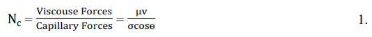
According to Barati-Harooni, et al., μ, v, σ, and θ stand for viscosity, velocity, interfacial tension between oil and brine, and contact angle, respectively. An increase in capillary count will result in an increase in total oil production. Several EOR techniques are screened for each crude oil reservoir to determine which one provides the greatest NC. The EOR process is effective when a method is selected to raise the capillary number to four or five order of magnitude [6]. One important strategy for raising NC in EOR is IFT reduction [7]. The capillary number is also considered in the water/brine flooding process, which is the primary means of secondary recovery stage before EOR operations. To identify the most effective operating conditions, it is also crucial to look into the IFT variations in various scenarios.
Interfacial Tension and Machine Learning
The IFT between crude oil-brine systems is affected by different temperature, pressure, and injection brine compositions for each type of crude oil. The most effective method of obtaining actual values is through laboratory-based experimental measurement of the IFT. That isn't always easy, though, particularly when it comes to the high temperatures and pressures found in oil reservoirs. IFT measurement can be costly and time-consuming in certain situations. As a result, in these situations, using mathematical models and estimating techniques is very beneficial.
Numerous Machine Learning (ML) techniques, such as fuzzy interference systems, Artificial Neural Networks (ANN), Support Vector Machines (SVM), Response Surface Model (RSM), Genetic Programming (GP), and other various evolutionary algorithms, have been developed (some based on the surface tension of two liquids) and applied in predicting crude oil–brine IFT.
In a recent study, Menad, et al., presented two innovative and potent machine learning techniques for calculating the IFT of crude oil-brine systems: "Gradient Boosting Decision Tree (GBDT)" and "Adaptive Boosting Support Vector Regression (AdaBoost SVR)." With each of these two data-driven techniques, two different types of models have been created. Pressure (P), Temperature (T), and four parameters characterizing the characteristics of crude oil (specific gravity (SG), Total Acid Number (TAN), and brine (pH, NaCl equivalent salinity (Seq), are the six inputs in the first kind, whereas the second kind only deals with four inputs (pH, TAN, and seq are not included). Nevertheless, their research was restricted to brine with high salinity, which forms the basis of the current study [8].
In the current study, medium and low salinity brine has been subjected to the Gradient Boosting Decision Tree (GBDT) and Adaptive Boosting Support Vector Regression (AdaBoost SVR) models. Additionally, additional parameters, such as polarizability per volume and dielectric constant, have been incorporated into the model to aid in its prediction of the impact of surfactants on the crude oil-brine IFT.
Role of Surfactants in Interfacial Tension Reduction
Often referred to as a surface-active agent, surfactants are substances like detergents that, when added to liquids lower their surface tension and improve their spreading and wetting capabilities. Surfactants aid in the uniform dye penetration of the fabric during textile dying. Aqueous suspensions of insoluble dyes and perfumes are dispersed using them. A portion of the surface-active molecule needs to be lipophilic (soluble in lipids or oils) and partially hydrophilic (soluble in water). In order to function as an emulsifying or foaming agent, it concentrates at the interfaces between bodies or droplets of water and those of oil, or fats [9].
Due to the ongoing depletion of conventional oil reserves and the sharp rise in the world's energy consumption, there is currently a great deal of interest in the various chemical Enhanced Oil Recovery (EOR) techniques. Chemical EOR is well-established with surfactant flooding as a method. This approach has shown to be effective because it uses a variety of mechanisms to improve oil recovery. They consist of emulsification, foam production, wettability modification, and Interfacial Tension (IFT) reduction. Surfactant flooding is still plagued by problems, such as excessive adsorption and instability in harsh or typical reservoir conditions, despite its widespread use. These problems have an impact on the anticipated oil recovery, which lowers the EOR projects' financial returns. However, surfactants can be chosen appropriately based on the type of rock and the conditions of the reservoir. Surfactant screening techniques are typically used for this, and they impose limits on the IFT, surfactant adsorption, and other factors under specific salinity and temperature conditions [10].
Time affects the Interfacial Tension (IFT) values between aqueous solutions and crude oil. Pre-equilibration of the oleic and aqueous phases does not completely eliminate changes with time, though this could be partially attributed to slow diffusion of certain components across the interface. IFT values that vary with interface age may also be caused by molecular rearrangement at the interface [11].
At very high or very low aqueous phase pH, reactions between the acidic and basic functional groups of heavier crude oil components can occur, producing in situ surfactants that can further change the IFT as a function of time. As noted by Bartell and Niederhauser and often observed since (e.g., Asekomhe, et al. and references cited therein), the gradual development of rigid films provides visible evidence of slow changes to the oil/brine interface [12].
According to research, low concentrations (∼0.05–0.2%) of various surfactant types can be used to achieve low interfacial tension, with values as low as 10-2 dynes/cm or less. When a surfactant is present in water without oil, it lowers surface tension because its molecules partially replace the water molecules at the water's surface. Less attraction exists between the molecules of surfactant and water than there is between the molecules of water. As a result, there is a decrease in the contraction force that causes surface tension [13]. On the other hand, in water-oil-surfactant systems, a process known as surfactant adsorption causes surfactant molecules to partially replace some of the water and oil molecules at the initial oil-water interface. The interaction between the surfactant's hydrophobic components and oil on one side of the interface and its hydrophilic components and water on the other is a result of this new arrangement of molecules. Actually, compared to the initial interaction between water and oil before surfactant addition, the new interaction across the oil–water interface is noticeably stronger. Consequently, there is a decrease in interfacial tension [14].
The kind and quantity of ions present in the brine have a significant impact on surfactants' capacity to lower the interfacial tension between crude oil and brine. As was previously mentioned, there is an ideal salinity at which the interfacial tension between brine and crude oil drops to extremely low levels. This ideal salinity is typically described in terms of the amount of dissolved NaCl in the solution [15]. Nevertheless, investigations revealed that the ideal salinity value is decreased when divalent or multivalent cations are added to a surfactant solution with a specific NaCl concentration. This indicates that the presence of these divalent/multivalent cations reduces the surfactant's tolerance to NaCl salinity, which has a negative impact on the interfacial tension between brine and oil. The impact of divalent cations on the interfacial tension characteristics of a surfactant formulation was examined in a study by Bansal and Shah. Both ethoxylated and petroleum sulfonates were present in the formulation. It has been shown that the ideal salinity of surfactant-oil-brine systems is significantly decreased when the concentration of divalent cations (Ca2+ and Mg2+) increases. Similar findings were made by Kumar et al., who demonstrated that surfactant solutions containing petroleum sulfonate and lignosulfonate would not be able to lower the oil-brine interfacial tension when Ca2+ and Mg2+ concentrations were increased.
Since these divalent cations are typically present in natural connate water, this effect should be taken into account during surfactant screening. This phenomenon is actually most commonly associated with anionic surfactants, which are known to precipitate out of the bulk solution when they react with divalent or trivalent cations. As a result, it is anticipated that oil recovery will be diminished [16].
Characterization of Surfactants
For technical and financial reasons, surfactants must be characterized. Verifying a surfactant's efficacy and stability over time is crucial before using it in any application.
Critical Micelle Concentration (CMC): According to Naseri, et al., and Bhosle, et al., a micelle is an aggregate form of surfactant molecules dispersed in a liquid colloid, as illustrated in Figure 1. The concentration of surfactant above which micelles can form is known as the Critical Micelle Concentration (CMC). Several of the solution's physicochemical characteristics, such as its viscosity, surface tension, and thermal and electrical conductivities, abruptly change at the CMC. Surfactant molecular structure (e.g., hydrophobic chain length), pressure conditions, solution salinity, ionic composition, pH, temperature, and other factors are some of the variables that affect a surfactant's CMC.

Figure 1: Micelle formation upon reaching the CMC
The CMC can be measured using more than thirty different techniques. These consist of the solubilization method, dye adsorption method, surface tension method, and others. Nesmerak and Nemcova have classified the methods used to measure the CMC into two categories: Direct methods and indirect methods. Through the use of direct methods, variations in surfactant concentration are seen to cause changes in certain properties of the surfactant solution. Consequently, the observed solution property, such as viscosity, electrical conductivity, refractive index, and slope change, is used to calculate the CMC. Conversely, indirect methods determine the CMC by monitoring a change in a particular property of a probe (a material added to the surfactant solution) in response to a variation in the surfactant concentration.
Nesmerak and Nemcova cite the voltammetric and spectrometric methods as examples of such techniques. IFT measurement is the most widely used technique to ascertain the CMC in surfactant EOR applications.
Hydrophilic–lipophilic balance: The Hydrophile–Lipophile Balance (HLB) is a crucial criterion for surfactant characterization. According to Kondo et al., and Reham et al., this criterion quantifies how lipophilic or hydrophilic a surfactant is. A surfactant's relative propensity to dissolve in water or oil is indicated by its HLB, which is a number on a scale from 0 to 20. A molecule made entirely of hydrophilic components has a value of 20, whereas a molecule that is completely hydrophobic (lipophilic) has a value of 0. Predicted surfactant properties based on HLB values are displayed in Table 1. Low-salinity formations require the selection of a low- HLB surfactant in order to form appropriate micro emulsions during oil recovery. Likewise, for formations with high salinity, a high-HLB surfactant ought to be chosen.
| HLB Value |
Property/application |
| 0-3 |
Anti-foaming agent |
| 04-06 |
W/O (Water in oil) emulsifier |
| 07-09 |
Wetting agent |
| 08-18 |
O/W emulsifier |
| 13-15 |
Detergent |
| 10-18 |
Hydro-trope or solubilize |
Table 1: Relation between HLB values and the expected properties/applications of surfactants.
Analysts created a few conditions for calculating the HLB values of surfactants. Investigate detailed by Griffin and Davies was among the most punctual inquire about to supply such conditions. Royer, et al. expressed Griffins condition for calculating the HLB for nonionic ethoxylated surfactants as follows:
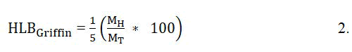
Where MH denotes the molecular mass of the hydrophilic part of the surfactant molecule and MT denotes the total molecular mass of the surfactant molecule. Royer et al., Davies discovered that group numbers can be used to calculate the HLB values of surfactants from their chemical formulae. As shown in the following equation:
molecular mass of the surfactant molecule. Royer et al., Davies discovered that group numbers can be used to calculate the HLB values of surfactants from their chemical formulae. As shown in the following equation:
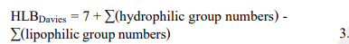
According to Davies, given a surfactant containing a number n of –CH2– groups, the HLB value is calculated as follows:
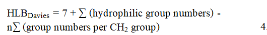
where Davies's tables are used to obtain the hydrophilic group numbers and the value of the CH2-group number is substituted with 0.475. Later, in order to ascertain the HLB values, additional researchers created experimental techniques. The Phase-Inversion Temperature (PIT), the Emulsion Inversion Point (EIP), and other techniques are the basis for some of these techniques.
Molecular Packing Parameter (MPP): The relationship between the geometry of a surfactant molecule and its aggregate structure in aqueous solutions is described by the term molecular packing parameter, or PC. Micelles in the form of spheres, rods, bilayer vesicles, etc. are examples of aggregate structures.
To calculate the PC, the following equation is used:
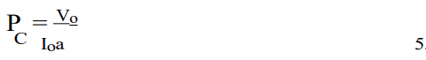
where vo is the volume of the surfactant tail, lo is the length of the surfactant tail, and a is the surface area of the hydrophilic head group at the surface of the aggregate. Figure 2 depicts the terms used in the equation of the packing parameter.

Figure 2: Definition of the terms used in equation of the packing parameter.
Different micelle geometries are formed by the surfactant molecules self-assembling based on the value of the packing parameter. These geometries have an impact on the solution's bulk characteristics, including its solubilization capacity and viscoelastic qualities.
Solubility ratio: The volume of oil (or water) solubilized per surfactant volume in a micro-emulsion phase is known as the oil (or water) solubilization ratio. The Solubilization Ratio (SR) can be expressed as follows, per Abalkhail, et al.:
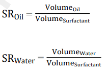
According to research by Bera, et al. and Hamidi, et al., SRwater and SRoil must be equal for the best solubilization to take place, which creates the perfect micro-emulsion formulation required for oil recovery [17]. Figure 3 illustrates how to obtain this by drawing the oil-SR curve and the water-SR curve, with the intersection point between the two curves representing the optimal solubilization occurring at the optimal salinity. According to Khaledialidusti, et al. and Liyanage, et al., understanding the solubilization parameters is crucial to optimizing the oil recovery process. This is due to the fact that optimal salinity is typically where the lowest oilwater IFT is found.

Figure 3: Intersection point between the two curves of SR-Oil and SR-Salinity.
Machine Learning Techniques
The branch of Artificial Intelligence (AI) known as Machine Learning (ML) focuses on creating systems that learn from the data they use and enhance their performance. The term artificial intelligence is used to describe a wide range of devices or systems that simulate human intelligence. Though the terms are sometimes used synonymously and are frequently discussed together, machine learning and artificial intelligence are not the same. The fact that not all AI is machine learning, even though all machine learning is, is a crucial distinction.
In various fields of study, various machine learning technologies have been presented in literature for parameter estimation, including Particle Swarm Optimization (PSO), Genetic Programming (GP), Artificial Neural Network (ANN), Imperialist Competitive Algorithm (ICA), and Generalized Regression Neural Networks (GRN).
Abooali, et al., used genetic programming for the first time to estimate IFT in crude oil-brine. Menad, et al., employed an empirical correlation as a system. Temperature, oil density, pressure, salinity, pH, and Total Acid Number (TAN) were among the input parameters. With an overall correlation coefficient (R2) of 0.9745, a root mean square error of 1.86 mN/m, and an average absolute relative deviation of 3.39%, the correlation's performance was very satisfactory [18].
In order to provide reliable, affordable, and quick paradigms for IFT prediction in crude oil-brine systems, Menad, et al. employed two data-driven techniques: "Adaptive Boosting Support Vector Regression (AdaBoost SVR)" and "Gradient Boosting trees (GBDT)." These approaches were put into practice and verified. In order to achieve this, a sizable data bank (560 data sets) was taken into consideration. These data sets covered a wide range of reservoir conditions, including Pressure (P) and Temperature (T), as well as the characteristics of crude oil, brine, and total acid number (TAN, SG, and pH). Using each of the aforementioned data-driven techniques, two types of models were implemented based on the inputs of the collected data. Six inputs are taken into account in the first kind, and four inputs (minus pH and TAN) are included in the second. Various statistical assessment criteria and graphical error analyses were used to assess the strength and suitability of the proposed models in predicting IFT of crude oil-brine systems and compare their results with the established correlations. Furthermore, a trend analysis was carried out on the most developed model to thoroughly assess its efficacy in comprehending how the variables used affected the IFT values.
Ultimately, the Leverage approach was employed to ascertain the predictive capability of the optimal model and to identify potential ambiguous data. There exist noteworthy disparities between this investigation and other previously published works in this particular domain: (1) Novel categories of machine learning (ML), namely Gradient Boosting trees (GBDT) and Adaptive Boosting Support Vector Regression (AdaBoost SVR), were utilized to establish more precise frameworks for Forecasting Interfacial Tension (IFT), (2) Two distinct scenarios were examined for each ML technique, taking into account various input parameters, and (3) The developed models are not only applicable for estimating IFT of pure components in brine, but also for predicting IFT between crude oil and brine.
Turgay and Qian reached the conclusion that although various AI techniques have achieved success in predicting petroleum reservoir properties, the knowledge and insights obtained from current research and applications suggest that intelligent models cannot fully substitute traditional reservoir engineering models, such as high-precision numerical simulators and analytical tools. However, the review provided no insight into the difficulties that arise when attempting to tap into the significant hydrocarbon reserves that are naturally confined within unconventional oil and gas reservoirs. This particular aspect is of utmost importance when it comes to the development of advanced AI models [19].
In order to model the surfactant enhanced drying of poly (styrene)-p-xylene coatings, Raj et al., employed a machine learning technique based on a regression tree. The developed model based on regression trees shows very good agreement between its predictions and the experimental data. Through experimentation, 16,258 samples in total were obtained. These samples were divided into two groups: 3298 samples were used to assess the prediction accuracy of the regression tree, and 12,960 samples were used to train the tree. Regression tree growth was done using MATLAB software. 8.8415 *10-6 was determined to be the mean squared error between the actual outputs and the values predicted by the model. He model exhibits strong generalization capabilities as it accurately predicts weight loss based on specific values of time, thickness, and triphenyl phosphate. Furthermore, it demonstrates a maximum error of only 1%. Its robustness allows it to be applied to various compositions and thicknesses within the system, thereby significantly minimizing the necessity for additional experiments to elucidate diffusion and drying processes.
In their study, Seddon, et al. employed a hybrid machine learning approach to forecast the surface tension profiles of hydrocarbon surfactants in aqueous solutions. The researchers proposed this approach based on the recognition that predicting the surface tension-log (c) profiles of hydrocarbon surfactants in aqueous solutions is not an easy computational task. This difficulty arises from the intricate and diverse architecture and interactions of surfactant molecules, making it empirically challenging as well [20].
Three characteristic parameters (Γmax, KL, and Critical Micelle Concentration, or CMC) were extracted from a datasets of SFT for 154 model hydrocarbon surfactants at 20–30 C by fitting it to the Szyszkowski equation. These parameters are correlated to a number of 2D and 3D molecular descriptors. After subtracting co-correlation, key (~10) descriptors were chosen, and Recursive Feature Elimination (RFE) was performed using a gradient-boosted regressor model to rank feature importance. To increase prediction accuracy and decrease over-fitting, the hyper-parameters of each target-variable model were adjusted through a randomized cross-validated grid search. With an R2=¼ 0.69-0.87 favorable correlation between the ML models and test experimental data, the approach's advantages and disadvantages are examined based on hydrocarbon surfactants that are "unseen." By adding a knowledge-based framework, the experimental data can be appropriately smoothed, making the data-driven approach more straightforward and broadly applicable.
Materials and Methods
For the present study, a set of 300 data points was collected from literature. These data contain interfacial tension of oilbrine systems, Pressure (P), Critical Miselle Concentration (CMC), Temperature (T), surfactant molecular packing parameter, surfactant HLB, and solubility ratio, KCl and MgS (Seq). The GBDT (Gradient Boosting Decision Tree) and the ADABOOST SVR (Adaptive Boosting Support Vector Regressor) algorithms where implemented with the collected data to predict the crude oil brine interfacial tension by developing two models for each of the algorithms and evaluated them using statistical parameters (Root Mean Square Error (RMSE), Coefficient of determination (R2), Average Absolute Relative Deviation (AARD) and Standard Deviation (SD)) to determine the best model to use for API development.
The first AdaBoost model (Model-1) was fitted with 5 input parameters (Interfacial Tension (IFT), Critical Micelle Concentration (CMC), Solubility Ratio (SR), Molecular Packing Parameter (MPP) and Hydrophilic–Lypophilic Balance (HLB)) with IFT set as the target variable. The hyper-parameters were tuned accordingly to obtain the best generalization for the model
Since the AdaBoost algorithm can be used for classification and regression, both algorithms were explored to determine which will perform better with the available data set. The regression model performed better with an accuracy of 84%.
The AdaBoost model-2 was implemented using a regressor algorithm and added two new surfactant parameters (density and molecular weight) to the five of model 1. An algorithm known as a regressor uses a given output to predict a continuous numerical value, in this case the IFT. A collection of characteristics or variables that are connected to the output value can be the input. Neural networks, decision trees, and linear regression are a few examples. The kind of output that a classifier and a regressor generate is the primary distinction between them.
The GBDT models were developed with similar alternations of the variables as that of the AdaBoost algorithm. The model one was fitted with 5 variables while the model 2 was fitted with 7 variables and the hyper-parameters tuned accordingly. The models of both the AdaBoost and the GBDT were evaluated using the previously mention performance metrics. The results of the evaluation metrics were compared with those from previous programs from literature to ascertain their competitiveness and authenticity.
Web application was developed using python with the flask API to connect the trained machine learning model to the user interface developed with HTML. The user interface connects the end user to the ML model while the flask API connects the user interface to the ML model.
Results and Discussion
A statistical measure frequently used in machine learning to assess a regression model's performance is the coefficient of determination (r2). It is a metric for assessing how well the data fit the regression line. Higher values denote a better fit. The range is 0 to 1. A model that perfectly fits the data is indicated by an r2 value of 1, while a model that does not explain any variability in the data is indicated by a value of 0. The r2 values for each of the developed models are displayed in Figure 4 below.

Figure 4: Performance summary of models.
Comparing the results of the GBDT models we see that the GBDT model-2 gave a better performance in predicting the IFT with an R2 of 99%
The R2 values of the GBDT model-2 and AdaBoost model-2 obtained in this study are compared to those of previous correlations and comparable machine learning models in Figure 5. Our GBDT model-2 has an r2 value of 0.9941 against 0.9967, which is still very good, ranking second to that of Amar et al.

Figure 5: R2 value comparison of models.
Cross-plots can be used to evaluate the model's generalization performance. It is a sign that the model is over fitting to the training data and may not generalize well to new, unseen data if the model performs significantly better on the training dataset than it does on the testing dataset. Conversely, if the model's performance on the training and testing datasets is similar, it suggests that the model is not over fitting and could potentially generalize well to new data (Figure 6). To enhance the model's generalization performance, we can experiment with different algorithms or modify the model's hyper parameters by examining the cross plots (Supplementary Table).

Figure 6: Comparison between predicted and experimental IFT computed from the model-2 of the GBDT algorithm with the predicted target variables IFT, SR, MPP, MW, Density and CMC. The blue dashed line corresponds with the slope.
From Figure 7, it can be seen that the fitted line in the GBDT model-2 tracks mostly actual data points, further demonstrating the high prediction performance of this approach.

Figure 7: Comparison between predicted and experimental IFT computed from the model-2 of the AdaBoost algorithm with prediction R2 score of 0.84.
On the other hand, model-2 of the AdaBoost algorithms data points are far apart from the fitted line implying a lesser accuracy compared to the former as shown in Figure 7.
One other way to gauge a machine learning model's accuracy is to look at its average absolute relative deviation, or AARD. It's a metric for assessing how accurately the model predicts the intended variable. The average of the absolute differences, divided by the actual values, between the predicted and actual values is known as the AARD. This works model is contrasted with literary models in the chart below (Figure 8).

Figure 8: Comparison between this study’s best models and other correlations.
The AARD is a useful metric because it measures the relative error, rather than the absolute error. This means that it is insensitive to the scale of the target variable, and can be used to compare the performance of models that predict different units of measurement. A lower AARD value indicates better accuracy of the regression model, as it indicates that the predicted values are closer to the true values.
A statistical tool for estimating the degree of variability or dispersion in a set of data is the standard deviation. The standard deviation specifically calculates the degree to which the data deviates from the mean or average. The standard deviation in regression analysis can be used to evaluate how well the model predicts the future. As can be seen in Figure 9, the GBDT model-2 yielded the lowest standard deviation of all the developed models, indicating low variability and high prediction accuracy.

Figure 9: Standard deviation values of the developed models.
The AdaBoost models produced the highest SD values, with model 1 performing the worst with 0.5385. A smaller standard deviation suggests that the model's predictions are more accurate and consistent, while a larger standard deviation would indicate that the model's predictions are more variable and less accurate. Based on the metrics results, it is evident that the GBDT algorithm outperforms the AdaBoost algorithm in terms of overall performance.
Here is a cross-section of the model's predicted values compared to the actual IFT values found in the literature to further demonstrate the GBDT model-2's prediction accuracy. A sample prediction of the model based on the available dataset is shown in Table 2 below. The very small deviations are evident, which is further consistent with the performance metrics analysis's findings. A graphical representation of the prediction accuracy is shown in Figure 10.
Table 2 indicates that the sample data's total deviations account for approximately 7.5% of the total predictions. This consistently translates into an accuracy of 93%, which is consistent with the 99.7% R2 result for the entire dataset's prediction accuracy. The GBDT model-2's prediction accuracy with only one significant deviation is graphically illustrated in Figure 10.
| Experimental values |
GBDT model-2 predictions |
Deviations |
| 0.007 |
0.003 |
0.0011 |
| 0.0031 |
0.0028 |
0.0003 |
| 0.0026 |
0.0026 |
0 |
| 0.352 |
0.28 |
0.072 |
| 0.0082 |
0.0082 |
0 |
| 0.0026 |
0.00258 |
0.0002 |
| 0.035 |
0.0338 |
0.0012 |
| 1.3 |
1.3 |
0 |
| 4.4 |
4.4 |
0 |
Table 2: Comparison of prediction of the GBDT model-2 with actual experimental values.
Based on its performance in all metrics, the GBDT model 2 is the best model; its deployment in an industrial environment comes next. This can be accomplished in a few ways, though they are outside the purview of this study: By integrating the model with already-existing software or systems; by establishing infrastructure to support the model; by making sure the model can process incoming data in real time; or by creating a mobile or web application specifically for the model. Creating the User Interface (UI) as well, so that people can communicate with the model. A simple web application was developed to demonstrate the models capability using flask API and a user interface with HTML. The homepage of the web app is shown in Figure 10.

Figure 10: Comparison of predicted and actual IFT values of the GBDT model.
Conclusion
The objective of this work was to use surfactant properties together with their crude oil/brine IFT data to create widely applicable, affordable, and accurate models for predicting crude oil-brine IFT. For this, "Gradient Boosting Decision Tree (GBDT)" and "Adaptive Boosting-Support Vector Regression (AdaBoost SVR)" are two potent machine learning techniques. During the modeling phase, a database containing 300 data sets was used. Based on the inputs taken into consideration, two different types of models were created for both algorithms: The first model uses six inputs (CMC, MPP, SR, HLB, Density, and Molecular Weight), while the second model uses four inputs (all of the above except for Density and Molecular Weight). As previously indicated, four models were created using the AdaBoost algorithms, the GBDT, and the available data set. The definitions of these models are provided in section 3. The GBDT model-2 results allow for the drawing of the following conclusions:
- Surfactant properties data with their corresponding experimental crude oil/brine IFT values is effective in modelling a machine learning program to predict IFT values with the surfactant variables as input parameters for the trained model.
- Four different models (two for each algorithm) were proposed to predict the IFT of crude oil-brine system among which GBDT model-2 with six inputs was found to be the best model. The developed GBDT model-2 can predict the IFT with high level of precision (the overall AARD% of this model is 1.32%; R2 of 99.41% and RMSE of 0.103).
- The comparison between the outcomes of the GBDT models and those of preexisting correlations further confirmed the superiority of the algorithms as previously shown in works by Amar et al and Seddon et al.
References
- Abooali D, Sobati MA, Shahhosseini S, Assareh M (2019) A new empirical model for estimation of crude oil/brine interfacial tension using genetic programming approach. J Petrol Sci Eng. 173:187-196.
[Google Scholar]
- Abalkhail N, Liyanage PJ, Upamali KA, Pope GA, Mohanty KK (2020) Alkaline-surfactant-polymer formulation development for a HTHS carbonate reservoir. J Petrol Sci Eng. 191:107236.
[Google Scholar]
- Andersen PO, Evje S, Kleppe H (2014) A model for spontaneous imbibition as a mechanism for oil recovery in fractured reservoirs. Transp Porous Media. 101(2):299-331.
[Google Scholar]
- Alvarado V, Manrique E (2010) Enhanced oil recovery: An update review. Energies. 3(9):1529-1575.
[Google Scholar]
- Al-Khafaji AH, Abdul-Majeed GH, Hassoon SF (1987) Viscosity correlation for dead, live and undersaturated crude oils. J Pet Res. 1987;6(2):1-6.
- Asekomhe SO, Chiang R, Masliyah JH, Elliott JA (2005) Some observations on the contraction behavior of a water-in-oil drop with attached solids. Ind Eng Chem Res. 44(5):1241-1249.
[Google Scholar]
- Azodi M, Nazar AR (2013) Experimental design approach to investigate the effects of operating factors on the surface tension, viscosity, and stability of heavy crude oil-in-water emulsions. J Dispers Sci Tec. 34(2):273-282.
[Google Scholar]
- Bahramian A, Danesh A (2004) Prediction of liquid–liquid interfacial tension in multi-component systems. Fluid Phase Equilibria. 221(1-2):197-205.
[Google Scholar]
- Bansal VK, Shah DO (1978) The effect of divalent cations (Ca++ and Mg++) on the optimal salinity and salt tolerance of petroleum sulfonate and ethoxylated sulfonate mixtures in relation to improved oil recovery. J Am Oil Chem' Soc. 55(3):367-370.
[Google Scholar]
- Bera A, Kumar T, Ojha K, Mandal A (2013) Adsorption of surfactants on sand surface in enhanced oil recovery: Isotherms, kinetics and thermodynamic studies. Appl Surf Sci. 284:87-99.
[Google Scholar]
- Barati-Harooni A, Soleymanzadeh A, Tatar A, Najafi-Marghmaleki A, Samadi SJ, et al. (2016) Experimental and modeling studies on the effects of temperature, pressure and brine salinity on interfacial tension in live oil-brine systems. J Mol Liq. 219:985-993.
[Google Scholar]
- Bratovcic A, Nazdrajic S (2020) Viscoelastic behavior of synthesized liquid soaps and surface activity properties of surfactants. J Surfactants Deterg. 23(6):1135-1143.
[Google Scholar]
- Bhosle MR, Joshi SA, Bondle GM (2020) An efficient contemporary multicomponent synthesis for the facile access to coumarinâ?fused new thiazolyl chromeno [4, 3â?b] quinolones in aqueous micellar medium. J Heterocycl Chem. 57(1):456-468.
[Google Scholar]
- Chu YP, Gong Y, Tan XL, Zhang L, Zhao S (2005) Studies of synergism for lowering dynamic interfacial tension in sodium α-(n-alkyl) naphthalene sulfonate/alkali/acidic oil systems. J Colloid Interface Sci. 276(1):182-187.
[Crossref] [Google Scholar] [PubMed]
- Carbonell JG, Michalski RS, Mitchell TM (1983) An overview of machine learning. Mach Learn. 3-23.
[Google Scholar]
- Davies JT (1957) A quantitative kinetic theory of emulsion type, I. Physical chemistry of the emulsifying agent. InGas/Liquid and Liquid/Liquid Interface. Proceedings of the International Congress of Surface Activity. 1:426-438.
[Google Scholar]
- Das A, Nguyen N, Nguyen QP (2020) Low tension gas flooding for secondary oil recovery in low-permeability, high-salinity reservoirs. Fuel. 264:116601.
[Google Scholar]
- Dietterich TG (2000) Ensemble methods in machine learning. InInternational workshop on multiple classifier systems. Berlin, Heidelberg: Springer Berlin Heidelberg.
[Google Scholar]
- El-Sebakhy E, Sheltami T, Al-Bokhitan S, Shaaban Y, Raharja I, et al. (2007) Support vector machines framework for predicting the PVT properties of crude-oil systems. InSPE Middle East oil and gas show and conference. SPE.
[Google Scholar]
- Edrisi SA, Dubey RK, Tripathi V, Bakshi M, Srivastava P, et al. (2015) Jatropha curcas L.: A crucified plant waiting for resurgence. Renew Sustain Energy Rev. 41:855-862.
[Google Scholar]
Citation: John O, Udoh T, Emenka B (2025) Prediction of Crude Oil-Brine Interfacial Tension (IFT) Based on Surfactant Characteristics Using Artificial Intelligence. Br J Res. 12:118.
Copyright: © 2025 John O, et al. This is an open-access article distributed under the terms of the Creative Commons Attribution License, which permits unrestricted use, distribution, and reproduction in any medium, provided the original author and source are credited.