Interventional Cardiology Journal Open Access

Keywords

Fractional flow reserve; Multi-artery; Effect of down-stream artery stenoses on lMCA; Percutaneous coronary intervention; Quantitative coronary angiography

Introduction

Multi-artery FFR vs single-artery FFR

When the FFR method has been introduced [1], it had some virtues that rightfully placed it in the highest class of coronary stenosis assessment techniques. Rather than focusing on the stenosis itself, it deals with the consequences of the stenosis and it is defined as the remnant blood flow through the stenotic artery relative to the flow through the artery in its original non-stenotic state, under conditions of minimal microvascular resistance. Minimal microvascular resistance can be achieved either by pharmacologically induced hyperemia for the duration of the intracoronary pressure measurements (as in the basic FFR method [1]) or by limiting the measurements to the period of the temporal minimum of the microvascular resistance during part of the diastole (as in the iFR method [2]). Unless otherwise stated or implied, for comparison or other purposes (Appendices A and B), it will be assumed in this article that conditions of minimal microvascular resistance apply in the arterial scenarios under consideration.

By its basic definition, FFR is the ratio of the flow Q_s through the stenotic artery and the presumable flow Q_o through the artery in its precedent stenosis-free state:

FFR=Q_s /Q_o (1)

It was experimentally established [3] that stenotic arteries with FFR<0.75 should be treated by revascularization whereas the ones with 0.85

FFR was introduced as a single-artery stenosis assessment index. In the case of a single vessel disease (SVD) with the aortic pressure on the proximal side of a stenosis, FFR is termed the true FFR (FFR^true). FFR^true of an end artery under such conditions is obtained from numerical values of intracoronary pressure measurements [1]:

FFR^true=P_d /P_a(2)

P_a- mean aortic pressure

P_d - mean distal pressure

P_ais the mean aortic driving pressure that forces the blood through the stenotic artery via its associated microvasculature into a particular region of the myocardium. From pressure-resistance- flow calculations one gets [1]:

FFR^true=1/(1+R_s/R_mv) (3)

R_s - stenosis resistance

R_mv - microvascular resistance associated with the artery

As can be seen from equation (3), FFR^true is dependent on R_mv. In case of past myocardial infarction (MI), part of the supplied region of the myocardium has been lost, it turned into scar tissue and its activity and blood consumption ceased. Perhaps paradoxically, under the new circumstances, the amount of blood supplied by the stenotic artery may be sufficient to cover the needs of the remaining (smaller) part of the supplied region of the myocardium. Not evident at first sight, but this too is reflected in the expression of FFR^true in equation (3). Loss of part of the formerly supplied region of the myocardium means loss of some arteriolecapillary complexes (Appendix A and B). Since all these complexes are in a parallel configuration, a loss of some of them results in an increase of R_mv (in analogy with electrical resistors). This in turn reduces the denominator in equation (3) which results in a greater FFR^true, indicating improvement and possibly an adequate blood flow to the remaining part of the supplied region of the myocardium. This is one of the important virtues of the FFR approach but in this article only cases that involve no pathology in the microvasculature will be dealt with. The purpose of this restriction is not to lose the 'physiologic match' between the artery size and the extent of its natural perfusion region from which originates the resistive relationship between the geometrical viscous resistance of the epicardial artery stem and its associated microvascular resistance (Appendix B).

In the FFR approach collaterals are usually also taken into account. Collaterals to the distal segment of a stenotic artery raise P_d thus improving the condition of the artery and increasing FFR^true (Equation (2)). This article focuses on other salient features of FFR in the MVD arena and therefore for the sake of simplicity cases with collaterals will not be considered directly in the formulas. However, through the actual increase of FFR^true, indirectly collaterals do affect the multi-artery FFR by the elevated measured distal intravascular pressures. Also, only localized stenosis (ordinary and diffuse) will be considered in the article, diffuse stenosis involving the whole length of an artery will not be considered.

In its basic form, as a single-artery coronary stenosis severity index, the FFR^true approach accounts very well for SVD cases. Cases of two or more stenosis in the same artery are also successfully handled within the frame of the basic FFR approach [4]. FFR has demonstrated its superiority over the angiographic coronary stenosis assessment method in the famous FAME study [5]. In the FAME study however only very simple MVD cases were considered. Cases of stenotic LM artery as well as post CABG cases were excluded. Each MVD case consisted of two or three stenotic major arteries (LAD, LCx, RCA) that were each treated as a separate and independent SVD case by the very basic single-artery FFR approach.

When an MVD case cannot be decomposed into simple independent SVD cases, the basic single-artery FFR approach can no longer provide guidance for the practitioner in the assessment of coronary stenosis, because of the stenosis-stenosis interaction. An important example is a stenotic LM coronary artery and a concomitant downstream stenotic artery (LAD or LCx). In this case the flows in the LAD and LCx arteries are interdependent because of the stenosis-stenosis interaction with the LM coronary artery. An attempt to approximate the FFR^true of the LM artery (by the apparent FFR) within the basic single-artery FFR approach may be considered reasonable only when the stenosis-stenosis interaction is low (i.e. low downstream stenosis) [6-8].

In the general MVD case, in the presence of significant stenosisstenosis interaction, the single-artery FFR method is no longer valid, it is even misleading and one needs consequently to resort to the multi-artery FFR approach [9]. The multi-artery FFR approach has been introduced in order to cope with non-negligible stenosis-stenosis interactions in the coronary MVD arena. The method has been demonstrated by treating a 3-artery configuration of a stenotic LMCA and a concomitant stenotic downstream sizable 'daughter' artery (LAD or LCX artery) [9].

In this article the multi-artery FFR method is generalized and its applicability is extended to additional stenotic 3-artery configurations of sizable coronary arteries as well as to typical coronary 'mother'-'daughter' configurations. The multi-artery FFR of a 3-artery configuration of the type [stenotic conductance-artery]- [two end-arteries/only one stenotic] is in principle dependent on the ratio δ of the microvascular resistances of the two end-arteries (Section 3.2). This suggests a possible morphology-dependent variation of the multi-artery FFR formula from patient to patient as well as a variation from one stenotic 3-artery configuration to another within the same patient (should such a rare event take place). This article addresses the need to look into this issue and see if it compromises the practicability of the multi-artery FFR method. The meticulous studies of the numerical examples of stenotic 3-artery configurations of sizable coronary arteries in [9] and in this article (Sections 4.1 and 4.2) indicate however that the ratio δ of the microvascular resistances has practically an insignificant effect on the multi-artery FFR. This enables the practitioner to be eventually 'mathematics-free' during a PCI procedure (despite the abundance of mathematics in this article) and carry out the PCI 'armed' with just 3 pre-calculated numerical tables while assessing such 3-artery configurations, as will be shown in this article (see also Discussion).

Stenotic 3-Artery Configuration: Some Specific Considerations

In the formal introduction of the multi-artery FFR approach the stenotic LMCA-LAD-LCx configuration was used as an example [9]. In the calculations it was taken into account that the mean dimensions of the stems of the LAD and LCx arteries (length, radii and the rate of tapering) are very similar and that therefore the mean microvascular resistances associated with these arteries are equal [9]. In the present article, the multi-artery FFR method is generalized and its capability is extended to resolve not just the LMCA-LAD-LCx configuration but also other stenotic 3-artery configurations of sizable coronary arteries of a patient. The calculations are based in principle on the actual dimensions of the patient's epicardial artery stems rather than on their statistical mean values. These morphological data are needed in order to obtain eventually the ratio between the microvascular resistances associated with the two end arteries of the configuration (Appendix B). The morphological data however vary in practice from one configuration to another, even for the same patient (should the unfortunate patient have 2 such stenotic configurations…). The obvious question is how sensitive indeed are the multi-artery FFR calculations to variations of the ratio δ of the microvascular resistances of the two end-arteries of the configuration and does it affect the practicability of the multi-artery FFR method. This issue will be explored in this article in detail.

The stenotic 3-artery configurations of sizable arteries considered in this article meet the following 2 conditions:

1. Each configuration consists of a stenotic artery that is, or can be functionally regarded, a conductance-artery that leads to, or bifurcates into, two end-arteries of which one is stenotic and the other one is stenosis-free.

2. The proximal pressure in the stenotic conductance artery is equal to, or very close to, the aortic pressure.

The purpose for these restrictive conditions is the applicability of the method to a number of important 3-way arterial intersections in the epicardial network (e.g. a sizable stenotic 'daughter' artery that splits off a proximally stenotic sizable 'mother' artery) that are preceded by a non-stenotic artery that maintains nearly an aortic driving pressure all the way to the beginning of the configurational stenotic conductance artery. The most important configuration of this kind is the LMCA-LAD-LCx configuration with a stenotic LMCA and a stenotic LAD (or LCx) artery. There are however also other possible cases. For example, a 3-artery configuration consisting of a proximally stenotic LAD artery with a sizable stenotic first diagonal D₁ and a non-stenotic remainder of LAD with this whole configuration preceded by a non stenotic LMCA (Section 4.2). Since LMCA is stenosis-free in this case, disregarding its negligible geometrical viscous resistance, the aortic pressure is maintained all the way to proximal LAD and forms the driving pressure through the configuration. Similarly, a relevant 3-artery configuration can be a stenotic proximal LCx artery with a stenotic sizable first marginal M₁ and a non stenotic remainder of LCx artery with the configuration preceded by a non stenotic LMCA. There can be in principle also other relevant configurations not described here.

The advantage of dealing with 3-artery stenotic configurations of sizable arteries in which only one end artery out of two is stenotic is that usually such a configuration can be resolved in practice by a relatively simple 2-variable numerical tabulation [9]. Although an algebraic solution is available, if tables can be prepared well in advance of the PCI procedure, they offer the benefit of providing also immediate information about the greater picture like the sensitivity of the actual FFR (FFR^real) to variations of each of the FFR^true(1) and FFR^true(3) auxiliary variables (Figure 1 and Tables 1-3 in [9]). The very same tables yield immediate information regarding the resulting FFR^real of each artery of the configuration in case the practitioner considers revascularization of any stenotic artery of the configuration.

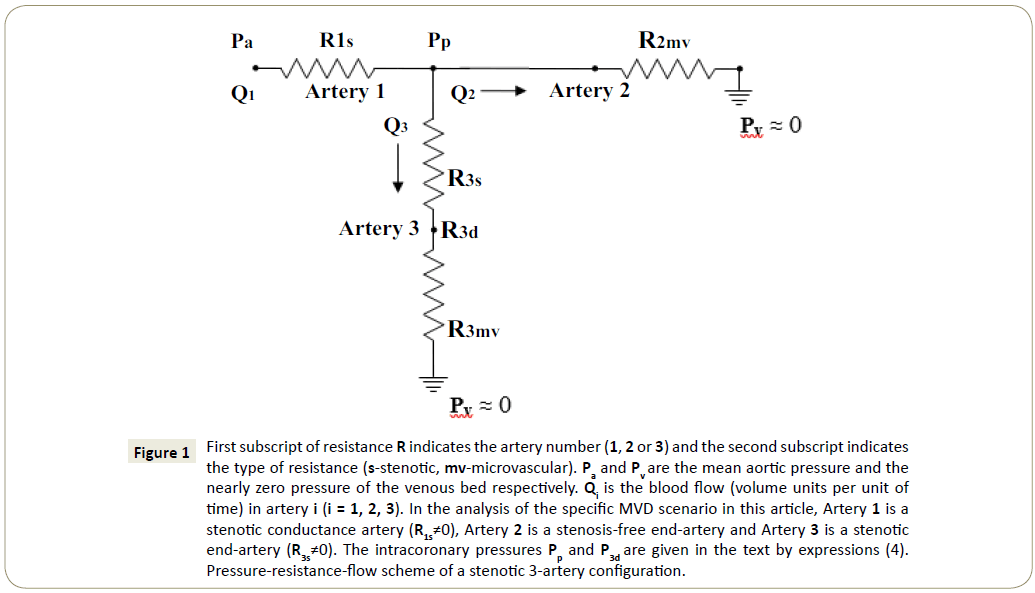
Figure 1: First subscript of resistance R indicates the artery number (1, 2 or 3) and the second subscript indicates the type of resistance (s-stenotic, mv-microvascular). P_aand P_v are the mean aortic pressure and the nearly zero pressure of the venous bed respectively. Q_i is the blood flow (volume units per unit of time) in artery i (i = 1, 2, 3). In the analysis of the specific MVD scenario in this article, Artery 1 is a stenotic conductance artery (R_1s≠0), Artery 2 is a stenosis-free end-artery and Artery 3 is a stenotic end-artery (R_3s≠0). The intracoronary pressures P_p and P_3d are given in the text by expressions (4). Pressure-resistance-flow scheme of a stenotic 3-artery configuration.

FFRtrue (LM)	FFRtrue (LAD)
	1	0.9	0.85	0.8	0.75	0.7	0.6	0.5	0.4	0.3	0.2	0.1	0
1	1	1	1	1	1	1	1	1	1	1	1	1	1
0.9	0.9	0.91	0.91	0.91	0.91	0.92	0.92	0.93	0.94	0.94	0.95	0.95	0.96
0.85	0.85	0.86	0.86	0.87	0.87	0.88	0.88	0.89	0.9	0.91	0.92	0.93	0.94
0.8	0.8	0.81	0.82	0.82	0.83	0.83	0.84	0.85	0.87	0.88	0.89	0.9	0.92
0.75	0.75	0.76	0.77	0.77	0.78	0.79	0.8	0.81	0.83	0.84	0.86	0.88	0.89
0.7	0.7	0.71	0.72	0.73	0.74	0.74	0.76	0.77	0.79	0.81	0.83	0.85	0.87
0.6	0.6	0.62	0.62	0.63	0.64	0.65	0.67	0.69	0.71	0.73	0.75	0.78	0.81
0.5	0.5	0.52	0.53	0.53	0.54	0.55	0.57	0.59	0.62	0.64	0.67	0.7	0.73
0.4	0.4	0.42	0.42	0.43	0.44	0.45	0.47	0.49	0.52	0.55	0.58	0.61	0.65
0.3	0.3	0.31	0.32	0.33	0.34	0.35	0.37	0.39	0.41	0.44	0.47	0.5	0.54
0.2	0.2	0.21	0.22	0.22	0.23	0.24	0.25	0.27	0.29	0.31	0.34	0.37	0.41
0.1	0.1	0.11	0.11	0.11	0.12	0.12	0.13	0.14	0.15	0.17	0.18	0.21	0.23
0	0	0	0	0	0	0	0	0	0	0	0	0	0
Calculated FFRapp (LM) (=FFRreal(LCx)=Q(s)LCx/Q(o)LCx)-under the influence of LAD-LM stenosis-stenosis interaction (Configurational microvascular resistance ratio δLAD/LCx=0.57)

Table 1: FFR^app(LM) is the apparent FFR(LM) that can be obtained by intracoronary FFR pressure measurements from the relationship FFR^app(LM)=P_p/ P_a. FFR^true(LAD) is also measurable, FFR^true(LAD)=P_3d/P_p. The FFR^app(LM) entries are different from FFR^true(LM) values of single LM artery because of the stenosis-stenosis interaction between LM and LAD arteries (LCx artery is stenosis-free). Note that LCx artery flow is affected too and that FFR^app(LM)= FFR^real(LCx) (see text). Q^(s)LCx is the LCx artery flow when LM and LAD arteries are stenotic while LCx artery is stenosis-free. Q^(o)LCx is the LCx artery flow when all 3 arteries are stenosis-free. The FFR^app(LM) values that constitute the first column of the table are FFR^app (LM)=FFR^true(LM) because they correspond to FFR^true(LAD)=1.00 (i.e. non-stenotic LAD artery). Note that within the FFR 'gray zone' the FFR^true table scale is expanded for both LM and LAD arteries. Values of FFR ≤0.2 never considered in practice are used in the table solely for mathematical illustration purposes.

FFRtrue (LM)	FFRtrue(LAD)
	1	0.9	0.85	0.8	0.75	0.7	0.6	0.5	0.4	0.3	0.2	0.1	0
1	1	0.94	0.9	0.87	0.84	0.81	0.75	0.68	0.62	0.55	0.49	0.43	0.36
0.9	0.9	0.85	0.82	0.8	0.77	0.74	0.69	0.63	0.58	0.52	0.47	0.41	0.35
0.85	0.85	0.8	0.78	0.76	0.73	0.71	0.66	0.61	0.56	0.5	0.45	0.4	0.34
0.8	0.8	0.76	0.76	0.72	0.69	0.67	0.63	0.58	0.54	0.49	0.44	0.39	0.33
0.75	0.75	0.71	0.69	0.68	0.66	0.64	0.6	0.56	0.51	0.47	0.42	0.37	0.32
0.7	0.7	0.67	0.65	0.64	0.62	0.6	0.56	0.53	0.49	0.45	0.41	0.36	0.31
0.6	0.6	0.58	0.56	0.55	0.54	0.53	0.5	0.47	0.44	0.4	0.37	0.33	0.29
0.5	0.5	0.48	0.47	0.47	0.46	0.45	0.43	0.41	0.38	0.36	0.33	0.3	0.27
0.4	0.4	0.39	0.38	0.38	0.37	0.37	0.35	0.34	0.32	0.3	0.28	0.26	0.24
0.3	0.3	0.29	0.29	0.29	0.28	0.28	0.27	0.26	0.25	0.24	0.23	0.21	0.2
0.2	0.2	0.2	0.2	0.19	0.19	0.19	0.19	0.18	0.18	0.17	0.17	0.16	0.15
0.1	0.1	0.1	0.1	0.1	0.1	0.1	0.1	0.1	0.09	0.09	0.09	0.09	0.09
0	0	0	0	0	0	0	0	0	0	0	0	0	0
Calculated FFRreal(LM)=Q(s)LM/Q(o)LM-under the influence of LAD-LM stenosis-stenosis interaction (Configurational microvascular resistance ratio δLAD/LCx=0.57)

Table 2: Q^(o)LM is the flow through the LM artery when LM, LAD and LCx arteries are stenosis-free. Q^(s)LM denotes the LM artery flow when LM and LAD arteries are stenotic while the LCx artery is stenosis-free. The FFR^real(LM) derivation method is described within the text. FFR^true denotes the familiar FFR of a single stenotic artery while all other arteries are stenosis-free. Note that within the FFR 'gray zone' the FFR^true table scale is expanded for both LM and LAD arteries. Also, the FFR^real(LM) of the first column of the table is equal to FFR^true(LM) because the column corresponds to non-stenotic LAD (i.e. FFR^true(LAD)=1.00). The low values FFR ≤ 0.2, never considered in practice, are used in the table just for mathematical trend indication.

FFRtrue (LM)	FFRtrue (LAD)
	1	0.9	0.85	0.8	0.75	0.7	0.6	0.5	0.4	0.3	0.2	0.1	0
1	1	0.9	0.85	0.8	0.75	0.7	0.6	0.5	0.4	0.3	0.2	0.1	0
0.9	0.9	0.82	0.77	0.73	0.69	0.64	0.55	0.46	0.37	0.28	0.19	0.1	0
0.85	0.85	0.77	0.73	0.69	0.65	0.61	0.53	0.45	0.36	0.27	0.18	0.09	0
0.8	0.8	0.73	0.69	0.66	0.62	0.58	0.51	0.43	0.35	0.26	0.18	0.09	0
0.75	0.75	0.69	0.65	0.62	0.59	0.55	0.48	0.41	0.33	0.25	0.17	0.09	0
0.7	0.7	0.64	0.61	0.58	0.55	0.52	0.45	0.39	0.32	0.24	0.17	0.08	0
0.6	0.6	0.55	0.53	0.51	0.48	0.45	0.4	0.34	0.28	0.22	0.15	0.08	0
0.5	0.5	0.46	0.45	0.43	0.41	0.39	0.34	0.3	0.25	0.19	0.13	0.07	0
0.4	0.4	0.37	0.36	0.35	0.33	0.32	0.28	0.25	0.21	0.16	0.12	0.06	0
0.3	0.3	0.28	0.27	0.26	0.25	0.24	0.22	0.19	0.16	0.13	0.09	0.05	0
0.2	0.2	0.19	0.18	0.18	0.17	0.17	0.15	0.13	0.12	0.09	0.07	0.04	0
0.1	0.1	0.1	0.09	0.09	0.09	0.08	0.08	0.07	0.06	0.05	0.04	0.02	0
0	0	0	0	0	0	0	0	0	0	0	0	0	0
Calculated FFRreal(LAD)=Q(s)LAD/Q(o)LAD-under the influence of LAD-LM stenosis-stenosis interaction (Configurational microvascular resistance ratio δLAD/LCx=0.57)

Table 3: FFR^real(LAD) can be obtained by pressure measurements from the relationship FFR^real(LAD)=P_3d/P_a(see text for tabulation method). FFR^true(LAD) is also measurable, FFR^true(LAD)= P_3d/P_p. Q^(o)LAD is the flow through the LAD artery when LM, LAD and LCx arteries are stenosis-free. Q^(s)LAD denotes the LAD artery flow when LM and LAD arteries are stenotic while the LCx artery is stenosis-free. FFR^true denotes the familiar FFR of a single stenotic artery while all other arteries are stenosis-free. Note that within the FFR 'gray zone' the FFR^true table scale is expanded for both LM and LAD arteries. Also, the FFR^real(LAD) of the first row of the table is equal to FFR^true(LAD) because the row corresponds to non-stenotic LM (i.e. FFR^true(LM)=1.00). Values of FFR ≤ 0.2, never considered in practice, are used in the table just for mathematical trend indication.

Note that stenotic 3-artery configurations with both end-arteries stenotic cannot be resolved by means of a simple 2-dimensional tabular method because they involve 3 auxiliary variables (FFR^true( 1), FFR^true(2) and FFR^true(3)) in addition to the microvascular resistance ratio δ associated with the two end-arteries (for δ, Section 3.2). Fortunately, δ can be practically set constant at δ=1 under certain circumstances thus enabling the use of a tabular method in the case of just one stenotic end artery in appropriate stenotic 3-artery configurations, as will be shown in this article.

The Multi-Artery FFR Method and the Effect of Microvascular Resistance

Essentials of the multi-artery FFR approach

In the following, some essentials of the multi-artery FFR approach in the assessment of a stenotic 3-artery configuration will be discussed. The configuration under consideration in this article is given in Figure 1.

It is in principle the type of configuration treated in the formal introduction of the multi-artery FFR approach [9]. However, the stenotic conductance artery (Artery 1 in Figure 1) does not necessarily originate from the aorta although its proximal pressure is taken to be the aortic pressure. Artery 1 of Figure 1 can be a stenotic LMCA but it might as well be a stenotic proximal LAD artery preceded by non stenotic LMCA, so that the aortic pressure is maintained all the way to the origin of LAD artery (disregarding the negligible geometrical viscous resistance of LMCA), combined with a stenotic sizable D₁ artery to form a '3-artery' configuration (proxLAD-D₁-remainingLAD). There are several 3-artery configurations (with proximal aortic pressure) occasionally encountered in the PCI practice that are appropriate for such multi-artery FFR application, some of which will be listed later on.

Prior to turning to multi-artery FFR formulas, let's present the mean pressures P_p and P_3d at two particular points of Figure 1 [9]. These mean pressures are expressed in terms of the appropriate resistances R the numerical subscripts of which indicate the artery number (1, 2, 3) whereas the letter subscripts indicate the type of resistance (s-stenotic, mv-microvascular):

P_p= P_a/{[(R_1s/R_3mv)/(R_3s/R_3mv+1)+R_1s/R_2mv]+1} (4)

P_3d= P_a/{(R_1s/R_3mv+R_3s/R_3mv)+(R_1s/R_2mv)( R_3s/R_3mv+1)+1}

P_p and P_3d are dependent on 3 variables: (R_1s/R_2mv), (R_1s/R_3mv) and (R_3s/R_3mv). In FFR terminology these intracoronary pressures are eventually expressed in terms of 3 other variables: FFR^true(1) and FFR^true(3) (FFR^true of Arteries 1 and 3 respectively in Figure 1) and the microvascular resistances ratio δ (δ=R_3mv/R_2mv). It should be noted that FFR^true denotes the familiar FFR of a single stenotic artery with all other arteries virtually stenosis-free. Within the multi-artery FFR approach, FFR^true of an artery can be regarded as the basic FFR of the artery (e.g. revascularization is taken to yield FFR^true=1.00 for the artery but it does not necessarily imply FFR^real=1.00). FFR^true of an artery is expressed in terms of stenotic and microvascular resistances precisely as in the single-artery FFR approach but because of stenosis-stenosis interaction FFR^true is no longer equal to the Q_s /Q_o of the artery (Q_s and Q_o are the actual flow through the artery and the flow through the artery in the virtual all-stenosis-free state respectively). FFR^true(1) and FFR^true(3) served as auxiliary variables by which the actual FFR, namely FFR^real=Q_s /Q_o , of each artery was expressed [9]. It should be also noted at this point that in the multi-artery FFR formal introduction article the microvascular resistances ratio variable δ was preset to δ=1 (R_3mv=R_2mv) and therefore the FFR^real characterization of each of the arteries forming the 3-artery configuration LMCA-LAD-LCx was practically dependent only on 2 variables, FFR^true(1) and FFR^true(3), enabling a tabular resolution [9]. Tables 1-3, that could be all prepared and kept ready prior to commencing a PCI procedure (Discussion), could yield the FFR^real condition of each artery and they could also yield the FFR^real condition of each artery upon virtually exercising each of the revascularization options. Perhaps an equally important virtue of the tables was their demonstration of the quantitative effect of the stenosis- stenosis interaction on each artery. Without this interaction, the FFR of each artery would remain at the basic level of FFR^true, as if all other arteries were stenosis-free. The tables showed that because of the stenosis-stenosis interaction, the FFR of each artery was transformed from its basic FFR^true value into the actual FFR^real value that could differ considerably from FFR^true. With a scale resolution of ΔFFR^true=0.02 (chosen by taking into account the accuracy level of the results in [9]), the tables are of a medium physical size and each could be prepared in advance in a hard-copy form for the practitioner to easily access each of the table elements during the PCI procedure.

The directly measurable FFR^real expressions of the arteries in Figure 1 of [9] were:

FFR^real(2)=FFR^app(1)=P_p/P_a(FFR^app denotes the apparent FFR) (5)

FFR^real(3)=P_3d/P_a(6)

FFR^real(1) was not directly measurable but it could be obtained from the following expression:

FFR^real(1)={ [1- FFR^app(1) ]/[1- FFR^true(1) ] } FFR^true(1) (7)

FFR^true(1) also could not be obtained directly. Since the numerical value of FFR^app(1) was known, therefore Table 1 of FFR^app(1) could be used in the search for FFR^true(1) [9].

As the very first step in the tabular method, the numerical value of FFR^app(1)=P_p/P_awas crossed with the numerical value of FFR^true(3)=P_3d/P_p in Table 1 to obtain the numerical value of FFR^true(1). Knowing FFR^true(3) and FFR^true(1), the value of FFR^real(1) could be then derived from Table 2 and the value of FFR^real(3) from Table 3.

With the FFR^real values of all the arteries in the configuration known, if not satisfactory, one could explore the potential effect of revascularization of artery 1 or artery 3, by setting the FFR^true of the revascularized artery in turn to 1.00 and using the appropriate tables and formulas [9]. The trivial option of revascularizing both arteries would always offer a possible resolution but that would be chosen only if the two stenotic arteries of the configuration were both highly stenotic and revascularization of just one of them would not sufficiently affect the other (through stenosisstenosis interaction) to result in acceptable FFR^real for all arteries of the configuration.

Microvascular Resistance Effect

In the formal introduction of the multi-artery FFR method [9], the method was applied to the stenotic LMCA-LAD-LCx arterial configuration, relying heavily on the statistical morphological similarity of the LAD and LCx arteries. Restricted consequently by the equality of the mean microvascular resistances associated with the LAD and LCx arteries, the multi-artery FFR method in that article could yield just general guidance for the PCI treatment of the LMCA-LAD-LCx configuration (Figure 2).

In this article however, without any dependence on statistics, the multi-artery FFR will be shown to have the capability of resolving 3-artery configurations of Figure 1 in any individual patient. The actual ratio δ of the microvascular resistances associated with patient's stenotic end artery 3 and non-stenotic end artery 2 (Figure 1) is regarded in the article as a configurational parameter. Given the morphological data of arteries 2 and 3, the detailed way of δ calculation is presented in Appendix A,

δ=δ_3/2=R_3mv/R_2mv → R_3mv= δ R_2mv (8)

It should be stressed at this point that the choice of artery notation in Figure 1 and in the mathematical equations and formulas in this article is not incidental: The stenotic end-artery in this article is always denoted artery 3 whereas the non-stenotic endartery is always denoted artery 2. In particular, it should be noted that δ of equation (8) is the ratio:

δ=[Microvascular resistance associated with stenotic end-artery]/[ Microvascular resistance associated with non stenotic end-artery]

Using the expression FFR^true(1)=1/(R_1s/R_2mv+R_1s/R_3mv+1) one gets

R_1s/R_2mv=[δ/(1+ δ)]Ã[1 – FFR^true(1)]/FFR^true(1)   (9)

R_1s/R_3mv=[1/(1+ δ)]Ã[1 – FFR^true(1)]/FFR^true(1)

Combining these expressions and FFR^true(3)=1/(1+R_3s/R_3mv) with equations (4), one has

FFR^app(1)=1/{[1/(1+ δ)]ÃÆ{[1 – FFR^true(1)]/FFR^true(1)}Ã[FFR^true(3)+ δ]+1}   (10)

With a value of δ=0.57, equation (10) is used to construct Table 1 of calculated apparent FFR of artery 1 (Figure 1), FFR^app(1), as a function of the auxiliary variables FFR^true(1) and FFR^true(3).

The current numerical values of FFR^app(1) and FFR^true(3) are always obtained from the experimental data

FFR^app(1)=P_p/P_a    (11)

FFR^true(3)=P_3d/P_p

In order to get the current numerical value of FFR^true(1) by the tabular method, the experimental value of FFR^app(1) is crossed with the experimental value of FFR^true(3) in Table 1 (calculated with δ=0.57 for the examples of section 4.1) and the user can readily figure out the numerical value of FFR^true(1) that corresponds to the crossing point.

FFR^true(1) can be also obtained algebraically from equation (10), using the data (11) and the appropriate value of δ:

FFR^true(1)=1/{[1/FFR^app(1) - 1]Ã(1+ δ)/[FFR^true(3)+δ]+1}    (12)

In the basic single-artery FFR method, FFR^true does reflect reality but not when a significant stenosis-stenosis interaction is present. Here the actual Q_s /Q_o ratio for an artery is given by FFR^real of the artery.

Equations (7) and (10) yield

FFR^real(1)={FFR^true(1)Ã[FFR^true(3)+δ]}/{[1-FFR^true(1)]ÃÆ[FFR^true(3)+δ]+ [(1+δ)FFR^true(1)]} (13)

Equation (13) is used to construct Table 2 of the calculated values of FFR^real(1) as a function of the auxiliary variables FFR^true(1) and FFR^true(3) for δ=0.57 (Section 4.1).

Similarly, equations (5) and (10) yield

FFR^real ( 2 ) = FFR^app ( 1 ) = 1 / { [ 1 / ( 1 + δ ) ] Ã { [ 1 – FFR^true( 1 ) ] / FFR^true(1)}[FFR^true(3)+δ]+1} (14)

Using equations (4), (9) and (6) one gets

FFR^real ( 3 ) = 1/{ [ 1 / ( 1 + δ ) ] Ã [ 1 - FFRt rue( 1 ) ] / FFRt rue( 1 ) + [ 1 / FFR^true(3)]{1+[δ/(1+δ)][1– FFR^true(1)]/FFR^true(1)}}    (15)

The calculated values of FFR^real(3) for δ=0.57 are listed in Table 3 as a function of FFR^true(1) and FFR^true(3) (Section 4.1).

Tables 1, 2 and 3 and the various algebraic expressions with δ=0.57 will be used to resolve the condition of the stenotic 3-artery configuration in section 4.1. All other configurations presented in this article will be resolved only by algebraic expressions, with the appropriate values of δ, since the tabular method has been already described at length elsewhere [9].

Assessing a Small Stenotic Side Branch

The multi-artery FFR method can be used not only to resolve the condition of appropriate 3-artery configurations but also to handle small stenotic branches splitting off sizable arteries. Coronary 'daughter' arteries are usually of a substantially smaller radius and therefore of much higher geometrical viscous resistance than their 'mother' arteries. Because of the proportionality relationship between the epicardial and associated microvascular resistances (Appendix A), the microvascular resistance associated with a 'daughter' artery is usually also much higher than that associated with its 'mother' artery. A stenotic 'mother' artery and a further downstream concomitant stenotic small 'daughter' artery is not an uncommon scenario.

The scheme of the 3-artery configuration of Figure 1 can be used to illustrate such a 'mother'-'daughter' scenario too. Artery 1 can be regarded as the stenotic segment of the 'mother' artery preceding the split-off point whereas artery 2 can be the non-stenotic remainder of the 'mother' artery. Artery 3 can represent the stenotic small 'daughter' artery. Under the circumstances, the ratio δ of the microvascular resistances in this scenario,

δ=δ_3/2=R_3mv/R_2mv (16)

can be relatively high, namely 1<< δ.

In order to assess the condition of each artery in this case, the FFR^real of the arteries should be approximated under the condition 1<<δ. The approximation process is mathematically simple, one takes δ to tend to infinity (δ→∞) in the various formulas, and the approximations are readily obtained.

Expression (13) yields

FFR^real(1) ≈ FFR^true(1)    (17)

1<<δ

The approximation of FFR^real(2) can be obtained from expression (14),

FFR^real(2) ≈ FFR^true(1) (18)

1<<δ

These approximations should have been expected since artery 2 in this scenario is the extension of the stenotic 'mother' artery 1 in Figure 1. Ordinarily, in the absence of strong stenosis-stenosis interaction, the small 'daughter' artery 3 has no effect on the sizable 'mother' artery, the opposite however is incorrect, as will be seen shortly.

FFR^real(3) under the condition 1<<δ can be approximated from expression (15),

FFR^real(3) ≈ FFR^true(1)FFR^true(3)   (19)

1<<δ

Expression (19) shows that the 'mother' artery (Arteries 1 and 2) does affect the 'daughter' artery 3. It should be noted that by the basic single-artery FFR approach, the 'daughter' artery 3 would be graded just by FFR^true(3) but by the multi-artery FFR method (which takes into account the actual flow through artery 3), the effect of the stenosis in the 'mother' artery does also manifest itself (by the presence of FFR^true(1) in expression (19)).

It should be noted that in practice the beginning of the high limit range 1<<δ for the numerical values of δ may depend on circumstances. If the stenosis in the stenotic 3-artery configuration are in the intermediate range of stenosis severity (usually of high interest to practitioners), even a value of about δ=8.6 may be considered as belonging to the high range 1<<δ, as far as the validity of the high limit approximations is concerned (Example #1). In case of a highly stenotic artery within the 3-artery configuration, a value of about δ=8.6 may not be high enough (for the high limit formulas to be valid) since the strong stenosis-stenosis interaction may give rise to a significant 'daughter' artery effect on the 'mother' artery (Example #2). It should be noted however that the range of 10<δ may already involve too tiny 'daughter' arteries with contraindication for PCI.

In order to make use of the FFR^real approximations made here, one needs to approximate the current numerical values of FFR^true( 1) and FFR^true(3) (in equations (17)-(19)) under the condition 1<<δ.

Formula (10) for FFR^app(1) yields FFR^app(1) ≈ FFR^true(1)   (20)

1<<δ

Therefore the approximation of the current numerical value of FFR^true(1) is

FFR^true(1) ≈ FFR^app(1)=P_p/P_a(21)

1<< δ

One has also FFR^true(3)=P_3d/P_p for any δ.

Using these expressions for the current values of FFR^true(1) and FFR^true(3), the numerical approximations of the current values of FFR^real(1), FFR^real(2) and FFR^real(3) are obtained:

FFR^real(1) ≈ P_p/P_a

1<< δ

FFR^real(2) ≈ P_p/P_a(22)

1<< δ

FFR^real(3) ≈ P_3d/P_a

1<< δ

These numerical approximations of the current values of FFR^real reflect the status of the 'mother' and 'daughter' arteries by which one can tell if revascularization is needed or if just medical therapy is sufficient.

The Microvascular Effect in Some Multi-Artery FFR Applications

The stenotic LMCA-LAD-LCx configuration

The stenotic LMCA-LAD-LCx configuration can be schematically represented by Figure 1 if one takes Artery 1 to correspond to stenotic LMCA, artery 2 to correspond to non-stenotic LCx and artery 3 to correspond to the stenotic LAD artery. The multi-artery FFR method should be in principle tailored to the morphology of the end arteries of the arterial configuration under consideration, the data of which will be listed here.

In order to obtain the ratio between the geometrical viscous resistances of the two end arteries (the stenotic LAD and non-stenotic LCx arteries) the following typical morphological data [10] will be used:

Stem of LAD: L_LAD=130 mm R_LADp=1.85 mm R_LADd=0.95 mm   (23)

Stem of LCx: L_LCx=80 mm R_LCxp=1.73 mm R_LCxd=0.65 mm (24)

Using the notation of Appendix A, one has

δ= δ_3/2=Res_3g/Res_2g=Res_LADg/Res_LCxg

δ={ L_LAD/[3R_LADp ³R_LADd ³/(R_LADp ²+R_LADpR_LADd+R_LADd ²)] }/ { L_LCx/[3R_LCxp³R_LCxd ³/(R_LCxp ²+R_LCxpR_LCxd+R_LCxd ²)] } (25)

Using the morphological data of typical LAD and LCx arteries listed here, the calculations yield δ=0.57 and this is the numerical value of δ that will be taken for the stenotic LMCA-LAD-LCx configuration considered in this section.

In order to demonstrate the effect of δ, for comparison purposes the same experimental intracoronary mean pressure values of Example #1 in [9] will be employed here too. The microvascular resistances associated with the LAD and LCx arteries there were taken to be equal, hence the δ used in that example was δ=1 [9]. In the example presented here, the calculated value of δ=0.57 will be used.

Example #1 is the first example to be presented here. The resolution will be by the tabular method with an algebraic corroboration.

δ=0.57

The mean pressure values to be used here will be the following:

P_a=100 mm Hg

P_p=86 mm Hg

P_3d=73 mm Hg

Table 1 of calculated FFR^app(LM) numerical values (with δ=0.57) can be obtained from expression (10) that assumes the following form for this example

FFR^app(LM)=1/{[1/(1+ δ)]{[1–FFR^true(LM)]/ FFR^true(LM)}Ã[FFR^true(LAD)+δ]+1}(26)

The current values of FFR^app(LM) and FFR^true(LAD) can be obtained from equations (11):

FFR^app(LM)=P_p/P_a=86/100=0.86

FFR^true(LAD)=P_3d/P_p=73/86=0.85

Crossing these numerical values in Table 1 (and corroborating by expression (12)) yields FFR^true(LM)=0.85 (also 0.85 for δ=1 in [9]).

By equation (5), FFR^real(LCx)= FFR^app(LM)=0.86 (also 0.86 for δ=1 in [9]).

Table 2 is constructed by formula (13):

FFR^real(LM)={FFR^true(LM)[FFR^true(LAD)+δ]}/{[1-FFR^true(LM)][FFR^true( LAD)+δ]+[(1+δ)FFR^true(1)]}

FFR^real(LM) derived from Table 2 (and corroborated by formula (13)), is FFR^real(LM)=0.78 (0.80 for δ=1 in [9]).

Formula (15) is used to construct Table 3 of FFR^real(LAD) numerical values:

FFR^real(LAD)=1/{[1/(1+δ)][1-FFR^true(LM)]/FFR^true(LM)+[1/ FFR^true(LAD)]{1+[δ/(1+δ)]Ã[1-FFR^true(LM)]/FF Rtrue(LM)}}

The numerical value of FFR^real(LAD), obtained from Table 3 (by using the numerical values of FFR^true(LM) and FFR^true(LAD)) and corroborated by the formula (15), is FFR^real(LAD)= 0.73 (also 0.73 for δ=1 in [9]).

The FFR^real(LM) and FFR^real(LAD) values in this case are obviously not satisfactory. This calls for revascularization measures. The trivial option of revascularization of both the LM and LAD arteries could definitely prove a solution but it would be, more often than not, inferior to a possibly successful option of having a revascularization of just one of these arteries that (through stenosis-stenosis interaction) would bring FFR^real of the other one to an acceptable level.

The FFR^real values will be therefore obtained from Tables 1,2 and 3 and corroborated algebraically for the following two revascularization options:

Option #1:Revascularization of LM, resulting in FFR^true(LM)=1.00 (with current FFR^true(LAD)=0.85)

Using the FFR^true values of the LM and LAD arteries, Table 2 and corroboration by formula (13) yield FFR^real(LM)=0.90 (0.93 for δ=1 in [9]).

FFR^real(LAD) can be obtained from Table 3 (with corroboration by formula (15)), FFR^real(LAD)=0.85 (also 0.85 for δ=1 in [9]).

FFR^real(LCx) is obtained from Table 1 (corroborated by formula (14)): FFR^real(LCx)=1.00 (also 1.00 for δ=1 in [9]).

Option #2:Revascularization of LAD, resulting in FFR^true(LAD)=1.00 (with current FFR^true(LM)=0.85)

Using the FFR^true values of the LAD and LM arteries, one gets the following results:

FFR^real(LM)=0.85 from Table 2 (corroborated by formula (13)) (also 0.85 for δ=1 in [9]).

FFR^real(LCx)= 0.85 is obtained from Table 1 and corroborated by formula (14) (also 0.85 for δ=1 in [9]).

From Table 3 one has FFR^real(LAD)= 0.85, corroborated by formula (15) (also 0.85 for δ=1 in [9]).

Numerically Option #1 seems preferable but if LMCA is unprotected, it implies a CABG operation which is not to be taken lightly. By the FFR^real values, Option #2 may be regarded nearly satisfactory and it seems that it can be regarded acceptable and preferable too, under the circumstances.

Example #2 will now be presented with the same intracoronary pressures of Example #2 of [9]. The resolution of this example will be made here by numerical tabulation with corroboration by the appropriate algebraic expressions.

δ=0.57

P_a=100 mm Hg

P_p=90 mm Hg

P_3d=27 mm Hg

Therefore:

FFR^app(LM)=90/100=0.90

FFR^true(LAD)=27/90=0.30

Crossing these two values in Table 1 (and corroborating by equation (12)) indicates that FFR^true(LM)=0.83 (0.85 for δ=1 in [9]).

Crossing this value with FFR^true(LAD)=0.30 in Table 2 (and corroborating by equation (13)), one gets FFR^real(LM)=0.50 (0.58 for δ=1 in [9]).

FFR^real(LCx) is given by FFR^real(LCx)=FFR^app(LM)=0.90 (Expression (14)) (0.90 for δ=1 in [9]).

FFR^real(LAD) can be obtained from Table 3 (corroboration by equation (15)), FFR^real(LAD)=0.27 (also 0.27 for δ=1 in [9]).

Obviously, the FFR^real(LM) and FFR^real(LAD) values indicate that the present condition of the configuration is unacceptable.

Revascularization options:

Option #1: Revascularization of LM, resulting in FFR^true(LM)=1.00 (with current FFR^true(LAD)=0.30 by initial intracoronary pressure measurements).

The FFR^real values of all 3 arteries can be obtained from Tables 1, 2 and 3 and also from the appropriate algebraic expressions:

FFR^real(LM)=0.5 (by Table 2 and expression (13)) (0.65 for δ=1 in [9]).

FFR^real(LCx)= 1.00 (by Table 1 and expression (14)) (also 1.00 for δ=1 in [9]).

FFR^real(LAD)= 0.30 (by Table 3 and expression (15)) (also 0.30 for δ=1 in [9]).

It is obvious that Option #1 is unacceptable.

Option #2: Revascularization of LAD, resulting in FFR^true(LAD)=1.00 (with current FFR^true(LM)=0.83 by initial intracoronary pressure measurements and Table 1), (FFR^true(LM)=0.85 for δ=1 in [9]).

The following FFR^real values can be obtained from Tables 1, 2 or 3 and corroborated by the appropriate algebraic expressions:

By Table 2 (and expression (13)): FFR^real(LM)=0.83 (0.85 for δ=1 in [9]).

By Table 1 (and expression (14)): FFR^real(LCx)=0.83 (0.85 for δ=1 in [9]).

By Table 3 (and expression (15)): FFR^real(LAD)=0.83 (0.85 for δ=1 in [9]).

Under the circumstances, Option #2 can be regarded as acceptable and the preferable course of action.

It should be noted at this point that in the range FFR^true(LM) ≥ 0.30 combined with FFR^true(LAD) ≥ 0.30, Tables 1, 2 and 3 of this article (for which δ=0.57) are almost identical to Tables 1, 2 and 3 respectively of the article of formal introduction of the multi-artery FFR [9] for which δ was δ=1. The preferable resolution options of the 3-artery configurations (with identical intracoronary pressures) are the same in the two articles (same FFR^real values to within ± 0.02) despite the different values of δ.

Stenotic proxLAD-D₁-remainderofLAD configuration (Sizable D₁)

The first diagonal artery D₁ can sometimes be a sizable artery that together with the LAD artery constitutes the stenotic '3-artery' configuration described in this section. It is assumed that the LMCA is stenosis-free so that the aortic pressure is maintained all the way to the origin of the proximally stenotic LAD artery (neglecting geometrical viscous resistance of the LMCA). The same morphology of the LAD artery stem used in section 4.1 will be used here as well. The artery configuration presented in Figure 1 can be used for the illustration of the configuration under discussion in this section: Artery 1=stenotic proximal segment of LAD, artery 2=non-stenotic remainder of LAD and artery 3=sizable stenotic first diagonal (D₁) artery.

Typical morphological data of a sizable stenotic fÃirst diagonal artery (D₁) is taken to be the following [10]:

Stem of D₁: L_D1=95 mm R_D1p=1.20 mm R_D1d=0.90 mm

Using the notation of Appendix A, one has

δ=δ_3/2=Res_3g/Res_2g=Res_D1g/Res_LADg

δ={L_D1/[3R_D1p ³ÃƒÆ’R_D1d ³/(R_D1p ²+R_D1pÃR_D1d+R_D1d ²)]}/ {L_LAD/[3ÃR_LADp³R_LADd ³/(R_LADp ²+R_LADpR_LADd+R_LADd ²)]}

It should be noted that D₁ is the stenotic end-artery here (and its data is therefore put in the numerator) whereas the remainder of the LAD artery is regarded as the non-stenotic end-artery.

Using the morphological data listed here, δ=1.72 and this is the numerical value of δ that will be taken for the proxLAD-D₁- remainderofLAD configuration in this section. Note that the geometrical viscous resistance of the non-stenotic remainder of the LAD artery is approximated here by the geometrical viscous resistance of the whole LAD artery. This is still a very good approximation because the geometrical viscous resistance per unit length of the proximal part of the LAD artery is negligible compared to that of the remainder of the LAD artery because of the relatively large arterial radius within the proximal segment.

In the following, two examples of stenosis assessment within the configuration under consideration will be presented for δ=1.72 with the same intracoronary pressures as in the two examples of section 4.1 of this article. For the purpose of comparison, the intracoronary pressures are also identical to those in the examples presented in [9].

Because of lack of space for additional tables, in this section the '3-artery' configuration will not be resolved by the tabular method but by the appropriate algebraic expressions.

Example #1 will be presented here with the following intracoronary mean pressures:

δ=1.72

P_a=100 mm Hg

P_p=86 mm Hg

P_3d=73 mm Hg

The current values of FFR^app(proxLAD) and FFR^true(D₁) can be obtained from Equations (11):

FFR^app(proxLAD)=FFR^real(remainder of LAD)=P_p/P_a=86/100=0.86

FFR^true(D₁)=P_3d/P_p=73/86=0.85

FFR^true(proxLAD) obtained from expression (12) is:

FFR^true(proxLAD)= 0.85 (also 0.85 for δ=1 in [9]).

This value of FFR^true(proxLAD) can be used in expression (13) in order to obtain FFR^real(proxLAD)=0.81 (0.80 for δ=1 in [9]).

Similarly, FFR^real(D₁) can be calculated by expression (15):

FFR^real(D₁)=0.73 (also 0.73 for δ=1 in [9]).

The FFR^real values of the proximal LAD and of the first diagonal artery D₁ indicate that a revascularization is required. The possibility of revascularization of just one of the two arteries will be explored here.

Option #1-revascularization of the proximal LAD artery, resulting in FFR^true(proxLAD)=1.00 (with FFR^true(D₁)=0.85).

By expressions (13) and (14),

FFR^real(proxLAD)= 0.94 (0.93 for δ=1 in [9]).

FFR^real(remainder of LAD)=FFR^app(proxLAD)=1.00 (also 1.00 for δ=1 in [9]).

Similarly, by expression (15),

FFR^real(D₁)= FFR^true(D₁)=0.85 (also 0.85 for δ=1 in [9]).

This option is evidently acceptable but Option #2 needs to be checked in order to conclude which one is preferable.

Option #2-revascularization of the D₁ artery, resulting in FFR^true(D₁)=1.00 (with FFR^true(proxLAD)=0.85).

Under this condition, the calculations yield

FFR^real(proxLAD)= 0.85 (also 0.85 for δ=1 in [9]).

FFR^real(remainder of LAD)=FFR^app(proxLAD)=0.85 (also 0.85 for δ=1 in [9]).

FFR^real(D₁)= 0.85 (also 0.85 for δ=1 in [9]).

This option seems acceptable too but Option #1 leaves LAD artery in a better condition than in Option #2, therefore Option #1 is preferable.

Example #2 will now be presented with the same intracoronary pressures of Example #2 of section 4.1 and of [9].

δ=1.72

P_a=100 mm Hg

P_p=90 mm Hg

P_3d=27 mm Hg

Therefore:

FFR^app(proxLAD)=FFR^real(remainder of LAD)=P_p/P_a=90/100=0.90

FFR^true(D₁)=P_3d/P_p=27/90=0.30

FFR^true(proxLAD) can be obtained from equation (12)

FFR^true(proxLAD)=0.87 (0.85 for δ=1 in [9]).

FFR^real(proxLAD) from equation (13) is:

FFR^real(proxLAD)=0.67 (0.58 for δ=1 in [9]).

FFR^real(remainder of LAD) is given by FFR^real(remainder of LAD)=FFR^app(proxLAD)=0.90 (Equation (14)) (also 0.90 for δ=1 in [9]).

FFR^real(D₁) can be obtained from equation (15),

FFR^real(D₁)=0.27 (also 0.27 for δ=1 in [9]).

By the FFR^real(proxLAD) and FFR^real(D₁) values, it is obvious that the condition of the configuration is unacceptable.

Revascularization options:

Option #1: Revascularization of proxLAD, resulting in FFR^true(proxLAD)=1.00 (with current FFR^true(D₁)=0.30).

FFR^real(proxLAD)=0.74 (by expression (13)) (0.65 for δ=1 in [9]).

FFR^real(remainder of LAD)=1.00 (by expression (14)) (also 1.00 for δ=1 in [9]).

FFR^real(D₁)= 0.30 (by expression (15)) (also 0.30 for δ=1 in [9]).

It is obvious that Option #1 is unacceptable.

Option #2: Revascularization of D₁, resulting in FFR^true(D₁)=1.00 (with FFR^true(proxLAD)=0.87).

By expression (13):

FFR^real(proxLAD)=0.87 (0.85 for δ=1 in [9]).

By expression (14):

FFR^real(remainder of LAD)=FFR^app(proxLAD)=0.87 (0.85 for δ=1 in [9]).

By expression (15):

FFR^real(D₁)=0.87 (0.85 for δ=1 in [9]).

By the FFR^real values of the arteries of the configuration, Option #2 can be regarded as an acceptable and the preferable course of action.

Stenotic proxLAD-D₁-remainderofLAD configuration (ordinary D₁)

Despite the title of this section and the specific numerical data used in it, the section and its formulas can be used for any common stenotic 'mother'-'daughter' arterial configuration in which the 'daughter' artery is a side branch much smaller than the 'mother' artery with a split-off point after the location of stenosis in the 'mother' artery.

In the configuration discussed in this section, the LAD artery is stenotic in its proximal part (Artery 1 in Figure 1) with the rest of LAD artery being stenosis-free (Artery 2 in Figure 1). The LAD artery is preceded by a non-stenotic LMCA so the LAD proximal pressure is the aortic pressure to a very good approximation. The LAD artery stem is morphologically identical to the one in sections 4.1 and 4.2. The stenotic first diagonal artery D₁ is of normal size (Artery 3 in Figure 1) and it is therefore much smaller than its LAD 'mother' artery [10].

The morphological data of a typical first diagonal artery (D₁) is taken to be [10]:

Stem of D₁ : L_D1=89 mm R_D1p=1.00 mm R_D1d=0.50 mm

Using the notation of Appendix A, one has

δ=δ_3/2=Res_3g/Res_2g=ResD₁g/Res_LADg

δ={ L_D1/[3ÃR_D1p³ÃƒÆ’R_D1d ³/(R_D1p ²+R_D1pÃR_D1d+R_D1d ²)] }/ {L_LAD/[3R_LADp³ÃƒÆ’R_LADd ³/(R_LADp ²+R_LADÆR_LADd+R_LADd ²)] }

Using the morphological data of the D₁ and LAD arteries (listed here and in section 4.1), the calculations yield δ=8.58 and this is the numerical value of δ that will be taken for the exact calculations concerning the proxLAD-D₁-remainderofLAD configuration considered in this section. The results will be then compared with those obtained from approximation formulas in the limit 1<< δ.

It should be noted that the geometrical viscous resistance of the non-stenotic remainder of the LAD artery is approximated here by the geometrical viscous resistance of the whole LAD artery. As indicated already in section, this is absolutely justifiable because the geometrical viscous resistance per unit length of the proximal part of the LAD artery is negligible compared to that of the remainder of the LAD artery because of the substantial radial difference.

In the following, two examples of stenosis assessment within the configuration under consideration will be presented for δ=8.58 (and then compared with approximations of section 3.3 for the limit 1<< δ) with the same intracoronary pressures as in the two examples of sections 4.1 and 4.2 of this article. The intracoronary pressures are also identical to those in [9]. Because of lack of space, the '3-artery' configuration here will be resolved only by algebraic expressions given in this article.

Example #1 presented with the same intracoronary pressures of Example #1 of sections 4.1, 4.2 and of [9].

δ=8.58

The intracoronary mean pressures in this example are:

P_a=100 mm Hg

P_p=86 mm Hg

P_3d=73 mm Hg

By equations (11), the current values of FFR^app(proxLAD) and FFR^true(D₁) are:

FFR^app(proxLAD)=FFR^real(remainder of LAD)=P_p/P_a=86/100=0.86

FFR^true(D₁) =P_3d/P_p=73/86=0.85

FFR^true(proxLAD) can be obtained from expression (12):

FFR^true(proxLAD)=0.86

This value of FFR^true(proxLAD) can be used in expression (13) in order to obtain FFR^real(proxLAD):

FFR^real(proxLAD) =0.85

If instead of using this exact formula with δ=8.58, one uses the approximations (17), (20) and (21) in the limit 1<< δ, then

FFR^real(proxLAD)≈FFR^true(proxLAD)≈FFR^app(proxLAD)=0.86

1<< δ

This is obviously a very good approximation of the calculated exact value of FFR^real(proxLAD) for δ=8.58.

Similarly, FFR^real(remainder of LAD)=FFR^app(proxLAD)=0.86, for δ=8.58.

In the limit 1<< δ, by approximations (18), (20) and (21) one has

FFR^real(remainder of LAD)=FFR^app(proxLAD)=0.86

1<< δ

which is equal to the calculated exact value of FFR^real(remainder of LAD) for δ=8.58 here.

Turning to FFR^real(D₁), expression (15) yields the exact value for δ=8.58:

FFR^real(D₁) =0.73.

In the limit 1<< δ, approximations (19) and (20) yield

FFR^real(D₁) ≈FFR^true(proxLAD)FFR^true(D₁) ≈FFR^app(proxLAD)FFR^true(D₁) =0.73

1<< δ

which is equal to the exact calculated value of FFR^real(D₁) for δ=8.58.

The FFR^real value of the first diagonal artery D₁ indicates that a revascularization is required. The possibility of resolving the '3-artery' configuration by revascularizing just one of the two stenotic arteries will be explored here.

Option #1-revascularization of the proximal LAD artery, resulting in FFR^true(proxLAD)=1.00 (with FFR^true(D₁) =0.85).

By expressions (13) and (14),

FFR^real(proxLAD)= 0.98 and

FFR^real(remainder of LAD)=FFR^app(proxLAD)=1.00 for δ=8.58.

In the limit 1<< δ one has

FFR^real(proxLAD)≈ FFR^true(proxLAD)=1.00

FFR^real(remainder of LAD)≈ FFR^true(proxLAD)=1.00

by expressions (17) and (18) respectively.

By expression (15) one has

FFR^real(D₁)=FFR^true(D₁)=0.85 for δ=8.58.

In the limit 1<< δ one also gets FFR^real(D₁)≈(1.00)(0.85)=0.85 by expressions (19) and (22).

This option is evidently acceptable but Option #2 needs to be checked in order to conclude which one is preferable.

Option #2-revascularization of the D₁ artery, resulting in FFR^true(D₁)=1.00 (with FFR^true(proxLAD)=0.86, as has been found in this example).

Under these conditions, the calculations yield for δ=8.58

FFR^real(proxLAD)=0.86 by expression (13)

FFR^real(remainder of LAD)=FFR^app(proxLAD)= 0.86 by expression (14)

FFR^real(D₁)=0.86 by expression (15).

In the 1<< δ limit one gets the same FFR^real values by using expressions (17), (18) and (19).

Option #2 seems acceptable too but Option #1 leaves LAD artery in a substantially better condition than in Option #2, therefore Option #1 is preferable.

Example #2 will now be presented with the same intracoronary pressures of Example #2 of sections 4.1 and 4.2 and of [9].

δ=8.58

P_a=100 mm Hg

P_p=90 mm Hg

P_3d=27 mm Hg

Therefore:

FFR^app(proxLAD)=FFR^real(remainder of LAD)=P_p/P_a=90/100=0.90

FFR^true(D₁)=P_3d/P_p=27/90=0.30

FFR^true(proxLAD) can be obtained from equation (12) for δ=8.58

FFR^true(proxLAD)=0.89

In the high limit of 1<< δ one has by approximation (Equation (21))

FFR^true(proxLAD)≈90/100=0.90

1<< δ

which is in very good agreement with the calculated exact value for δ=8.58.

We'll calculate now FFR^real(proxLAD) from equation (13) for δ=8.58

FFR^real(proxLAD)=0.83.

The high limit approximation (Equation (17)) yields

FFR^real(proxLAD)≈ FFR^true(proxLAD)≈0.90

1<< δ 1<< δ

This high limit FFR^real(proxLAD) approximation deviates significantly from the calculated exact value.

The deviation is partly due to the current δ value of δ=8.58. Under the circumstances of Example#2 here, this δ value is not sufficiently high to moderate the main effect of reduction of FFR^real(proxLAD) by the highly stenotic D₁, through the strong stenosis-stenosis interaction. For mathematical demonstration, calculations show that FFR^real(proxLAD)=0.84 for δ=10 and that FFR^real(proxLAD)=0.86 for δ=20, approaching mathematically the high limit (1<< δ) value of 0.90. It should be however noted in passing that usually for about 10<δ the 'daughter' artery is already so tiny that it is contraindicated for PCI.

FFR^real(remainder of LAD) is given by FFR^real(remainder of LAD)=FFR^app(proxLAD)=0.90 (Expression (14)).

In the high δ limit FFR^real(remainder of LAD) is given by (Equation (18))

FFR^real(remainder of LAD)≈ FFR^true(proxLAD)≈0.90

1<< δ in very good agreement with the calculated exact value.

FFR^real(D₁) for δ=8.58 can be obtained from Equation (15),

FFR^real(D₁) =0.27

In the limit 1<< δ, from approximations (22) one has

FFR^real(D₁)≈0.27

1<< δ in very good agreement with the calculated exact value for δ=8.58.

By FFR^real(D₁), it is obvious that the condition of the configuration is unacceptable.

Revascularization options:

Option#1: Revascularization of proxLAD, resulting in FFR^true(proxLAD)=1.00, (with FFR^true(D₁) =0.30).

FFR^real(proxLAD)=0.93 for δ=8.58 (by expression (13)).

FFR^real(proxLAD) ≈ FFR^true(proxLAD)=1.00 in the 1<< δ limit (by equation (17))

FFR^real(remainder of LAD)=1.00 for δ=8.58 (by expression (14))

FFR^real(remainder o fLAD)≈ FFR^true(proxLAD)=1.00 in the 1<< δ limit (Equation (18))

FFR^real(D₁)=0.30 for δ=8.58 (by expression (15))

FFR^real(D₁) ≈ FFR^true(proxLAD) FFR^true(D₁)=(1.00) (0.30) =0.30 in the 1<< δ limit (Equation (19))

It is obvious that Option #1 is unacceptable, in this case the first diagonal artery D₁ cannot be relieved indirectly.

Option #2: Revascularization of D₁, resulting in FFR^true(D₁)=1.00, (with FFR^true(proxLAD)=0.89 and the 1<< δ high limit value of FFR^true(proxLAD)≈0.90).

By expression (13) for δ=8.58, FFR^real(proxLAD)=0.89.

In the 1<< δ limit it is FFR^real(proxLAD)≈ FFR^true(proxLAD)=0.90.

By expression (14) for δ=8.58, FFR^real(remainder of LAD)=FFR^app(proxLAD)=0.89.

The 1<< δ high limit yields FFR^real(remainder of LAD)≈ FFR^true(proxLAD)=0.90.

By expression (15) for δ=8.58, FFR^real(D₁) =0.89.

In the 1<< δ limit it is FFR^real(D₁) ≈ FFR^true(proxLAD) FFR^true(D₁) =0.90.

By the FFR^real values of the arteries of the configuration, Option #2 is acceptable and clearly the preferable course of action.

Discussion

In the formal introduction of the multi-artery FFR the method was applied to the stenotic 3-artery configuration consisting of stenotic LMCA, stenotic LAD and non-stenotic LCx end-arteries [9]. The mean microvascular resistances associated with the LAD and LCx arteries were taken to be equal on the grounds of statistically very close morphological similarity of the two arteries [10,11]. With the ratio of the mean microvascular resistances of the end-arteries being consequently equal to 1, the actual FFR (denoted FFR^real) of each of the 3 arteries of the configuration was dependent on the two auxiliary variables FFR^true(LM) and FFR^true(LAD) [9]. Being based in part on dimensional mean values, the multi-artery FFR seemed capable of providing the practitioner with just general guidance. In real practice, however general guidance is not sufficient, the method is expected to provide a specific resolution tailored to each 3-artery stenotic configuration of the individual patient. To this end, the exact morphology of the two configurational end-arteries should be taken into account, in order to obtain the microvascular resistances ratio δ of their stems (Appendices A and B). However, dealing with the morphology of the two end-arteries in each PCI procedure would create a very undesirable mixture of elaborate angiographic dimensional measurements and calculations, in addition to the ordinary FFR intracoronary pressure measurements. As this might adversely affect the acceptance of the multi-artery FFR method in the PCI practice, this issue has been explored in depth in this article.

A careful examination of Table 1 (FFR^real(2)), Table 2 (FFR^real(1)) and Table 3 (FFR^real(3)) of [9] and of this article shows the following:

1) Despite the differences in the ratios of the microvascular resistances (δ=1 in [9] and δ=0.57, δ=1.72 in this article) the corresponding tables are almost identical. The tables associated with δ=0.57 and δ=1.72, when compared to the corresponding ones in [9], show a difference of corresponding table elements of not more than ±0.04 within the practical range of the FFR^true auxiliary variables, 0.3 ≤ FFR^true(1) and 0.3 ≤ FFR^true(3) in each table, and even less (± 0.02) within the intermediate stenosis severity range of each table. The 3 Tables of δ=1.72 have been calculated separately and taken into account but are not shown in this article. Just for comparison and for illustration purposes, the FFR^real numerical values of the table elements in the δ=1.72 tables for the extreme point FFR^true(1)=FFR^true(3)= 0.30 are: FFR^real(1)=0.27, FFR^real(2)=0.37 and FFR^real(3)=0.11.

2) In the presence of stenosis-stenosis interaction no artery retains its basic FFR^true, it is transformed into a different actual FFR^real. In Table 1 the FFR^real(2) of the non-stenotic artery 2 (which is also FFR^app(1)) is shown (Figure 1). It is clearly seen that FFR^real(2) decreases when Artery 1 is more stenotic (smaller FFR^true(1)) because part of the reduced blood output of artery 1 goes through artery 2. Also, FFR^real(2) increases when artery 3 is more stenotic (smaller FFR^true(3)) because the blood flows in artery 2 and artery 3 are competing with each other. In Table 2 it can be seen that FFR^real(1) naturally decreases when artery 1 is more stenotic and it also decreases when artery 3 is more stenotic because the outflow of artery 1 encounters then a higher total resistance. In Table 3 the FFR^real(3) naturally decreases when artery 3 is more stenotic and also when artery 1 (that provides its inflow) is more stenotic. The immediate conclusion from the very close similarity of the appropriate tables corresponding to δ=0.57, δ=1 and δ=1.72 is that in resolving stenotic 3-artery configurations of sizable arteries (like in [9]) there is practically no need to recalculate δ when going from one patient to another. One can simply use the 3 Tables of [9], with δ=1, (preferably with a finer scale resolution of ΔFFR^true=0.02 for the auxiliary variables FFR^true(1) and FFR^true(3), compatible with the accuracy of FFR^real of the arteries within the low and intermediate stenosis severity ranges) for obtaining FFR^real of each of the 3 arteries of the stenotic configuration: Table 1-FFR^real for non-stenotic end-artery 2, Table 2 -FFR^real for stenotic conductance artery 1, Table 3-FFR^real for stenotic end-artery 3-see all arteries in Figure 1).

The multi-artery FFR method has been applied in this article to two types of examples of stenotic 3-artery configurations in which intracoronary pressure measurement readings are identical to those obtained in Example #1 and Example #2 respectively of the article of formal introduction of the multi-artery FFR method [9]. The corresponding examples are marked accordingly in this article. There is an important difference between the two types of examples. In Example #1 of [9] the 2 stenotic arteries of the configuration are the conductance artery LMCA and the LAD endartery (their counterparts being artery 1 and artery 3 respectively in Figure 1). The stenosis severity of both stenotic arteries in this type of example is in the low-intermediate stenosis severity range (basic FFR^true=0.85). In Example #2 of [9] however the same 2 arteries are stenotic but while the stenosis of LMCA is in the low-intermediate severity range (basic FFR^true=0.85), the LAD artery by itself is extremely stenotic (FFR^true(LAD)=0.30). The same holds true for the corresponding examples and appropriate arteries in the 4.1 and 4.2 sections of this article.

It should be noted that unlike in [9], in this article the reason for suggesting the use of the FFR^real tables that correspond to δ=1 for handling stenotic 3-artery configurations of sizable coronary arteries in the multi-artery FFR method in PCI procedures, is entirely different. Despite the inequality of the microvascular resistances associated with the end arteries of different patients, the use of the FFR^real tables that correspond to δ=1 is suggested for the following reasons. In any stenotic 3-artery configuration of sizable coronary arteries with end arteries A and B, if A is stenotic and B is not, then δ=δ₁=R_Amv/R_Bmv. Let's assume (without loss of generality) that δ₁ > 1. If the roles of A and B are interchanged, namely if B is stenotic and A is not, then δ=δ2 =R_Bmv/R_Amv=1/δ₁<1. It is therefore evident that the relevant δ values are in the proximity of δ=1. Furthermore, as found from the examination of the tables and examples, maintaining δ constant at δ=1, the multi artery FFR method is accurate for stenotic 3-artery configurations with stenoses in the low and intermediate stenosis severity ranges (like in the examples of the type of Example #1) and less accurate for stenotic 3-artery configurations in the high stenosis severity range (like in Example #2-type examples). With the δ=1 tables the method can be applied to stenotic 3-artery configurations of sizable arteries within their statistical range of morphological variations (radii, rates of tapering and lengths) that roughly correspond to the range 0.6 ≤ δ ≤ 1.7. As indicated already, this range covers also the possibility of end-arteries switching 'roles' in a 3-artery configuration (e.g. LCx being stenotic and LAD being stenosis-free in the examples of section 4.1 which boils down to using the inverse of δ, δ= 1/0.57 =1.75, instead of δ=0.57 in those examples).

The restriction imposed on the 3-artery configurations subjected to the multi-artery FFR method in this article, of having just one stenotic end-artery, is not to be taken lightly. This has been the 'price' for using the tabular method which would be otherwise not feasible. However, 3-artery configurations with both endarteries stenotic are not less common [12]. In practice, circumstances are sometimes favorable and in such cases one of the end arteries may be of negligible stenosis and can be regarded as stenosis-free, enabling the use of a tabular method or alternately it may be extremely stenotic, calling clearly for revascularization that would reduce the problem to a 2-dimensional level. With this being said, the 'one stenotic end-artery' restriction nevertheless remains a downside. Although this issue can be in principle resolved, doing it and yet retaining user-friendly mathematics in the process might not be a trivial matter.

A very useful by-product of the multi-artery FFR analysis in this article is the applicability of the method to common stenotic 'mother'-'daughter' configurations (sizable 'mother' artery and relatively tiny 'daughter' artery branch) often encountered in the PCI practice. From the examples of section 4.3 it can be seen that stenosis-stenosis interactions can be very influential in these configurations too. The high limit (1<< δ) simple formulas of section 3.3 can be considered already valid for δ=8.58 in cases of low-intermediate stenosis severity (Example #1 in section 4.3). In the presence of strong stenosis-stenosis interaction (Example #2 in section 4.3) however, even a considerably higher numerical value of δ cannot offset the suppression of FFR^real(1) by the stenosis- stenosis interaction and the high limit (1<< δ) formulas are not valid. Furthermore, considering the normal sizes of the major coronary arteries, going beyond about δ~10 implies tiny side branches that are already contraindicated for PCI. This however does not constitute a hindrance since the only stenotic 'mother'- 'daughter' configurations of interest to the practitioner, also for FFR application, are usually the ones with stenoses in the lowintermediate severity ranges (cases like Example #1 in section 4.3) and in these configurations the high limit (1<< δ) formulas of section 3.3 are valid and can be readily used.

The multi-artery FFR method, perhaps despite the first impression created by the abundance of mathematical expressions in this article, involves no direct mathematics at all on the part of the practitioner in the assessment of 3-artery configurations dealt with in this article during the PCI procedure. All that the practitioner should do in real time is to apply the tabular method in order to assess the current condition of the 3-artery configuration and to evaluate the outcome of possible revascularization options. The creation of hard copies of the 3 FFR^real tables (with δ=1 and of resolution ΔFFR^true=0.02) is an advance act performed only once and the tables are then applicable to an appropriate stenotic 3-artery configuration of sizable coronary arteries (like in Example #1 in sections 4.1 and 4.2). It should be noted at this point that attempting a finer scale resolution of ΔFFR^true=0.01 would not be justifiable on the grounds of accuracy within the δ range under consideration and would result in physically very large and inconvenient tables that the practitioner would need to move across a computer screen in order to access individual table elements. The mathematics in this article is even simpler when dealing with stenotic 'mother'-'daughter' configurations (like in Example #1 in section 4.3) that are resolved by the high limit (1<< δ) FFR^real very simple formulas (22) obtained directly from the measured intravascular pressure readings (see section 3.3) that to some extent can remind the reader of the simplicity of the mathematics of the basic single-artery FFR method.

This article opens the way for a wide use of the multi-artery FFR method, by FFR and iFR techniques, in accurate resolutions of appropriate stenotic 3-artery configurations of sizable arteries and appropriate stenotic 'mother'-'daughter' configurations commonly encountered in the PCI practice. There is no more need to use single-artery FFR approximations in such cases since they are valid only in the very low stenosis severity limit [6-8] but prove erroneous and even misleading in the intermediate and high stenosis severity ranges [9]. The multi-artery FFR method can be applied to these configurations in the low-intermediate stenosis severity ranges with an accuracy of better than ± 0.02 for FFR^real of the constituent arteries (Example#1-type examples of sections 4.1, 4.2 and 4.3).

References

1. Pijls NH, van Son JA, Kirkeeide RL, de Bruyne B, Gould KL (1993) Experimental basis of determining maximum coronary, myocardial, and collateral blood flow by pressure measurements for assessing functional stenosis severity before and after percutaneous transluminal coronary angioplasty. Circulation 87: 1354-1367.
2. Nijjer SS, Sen S, Petraco R, Davies JER (2015) Advances in coronary physiology. Circulation J. 79: 1172-1184.
3. Petraco R, Sen S, Nijjer S, Echvarria-Pinto M, Escaned J, et al. (2013) Fractional flow reserve-guided revascularization-practical implications of a diagnostic gray zone and measurement variability on Clinical Decisions. J Am Coll Cardiol Intv 6: 222-225.
4. Pijls NHJ, De Bruyne B, Bech GJW, Liistro F, Heyndrickx GR, et al. (2000) Coronary pressure measurement to assess the hemodynamic significance of serial stenoses within one coronary artery-validation in humans. Circulation 102: 2371-2377.
5. Tonino PAL, de Bruyne B, Pijls NHJ, Siebert U, Ikeno F, et al. (2009) Fractional flow reserve versus angiography for guiding percutaneous coronary intervention. N Engl J Med 360: 213-224.
6. Daniels DV, Van't Veer M, Pijls NHJ, van der Horst A, Yong AS, et al. (2012) The impact of downstream coronary stenoses on fractional flow reserve assessment of intermediate left main disease. J Am Coll Cardiol Interv 5: 1021-1025.
7. Yong ASC, Daniels D, de Bruyne B, Kim HS, Ikeno F, et al. (2013) Fractional flow reserve assessment of left main stenosis in the presence of downstream coronary stenoses. Cir Cardiovasc Interv 6: 161-165.
8. Fearon WF, Yong AS, Lenders G, Toth GG, Dao C, et al. (2015) The impact of downstream coronary stenosis on fractional flow reserve assessment of intermediate left main coronary artery disease. J Am Coll Cardiol Intv 8: 398-403.
9. Yaeger IA (2016) A multi-artery fractional flow reserve (FFR) approach for handling coronary stenosis-stenosis interaction in the multi-vessel disease (MVD) arena. Int J Cardiol 203: 807-815.
10. Dodge Jr. JT, Brown BG, Bolson EL, Dodge HT (1992) Lumen diameter of normal human coronary arteries-influence of age, sex, anatomic variation, and left ventricular hypertrophy or dilation. Circulation 86: 232-246.
11. Zhang LR, Xu DS, Liu XC, Wu XS, Ying YN, et al. (2011) Coronary artery lumen diameter and bifurcation angle derived from CT coronary angiographic image in healthy people (Article in Chinese). Zhonghua Xin Xue Guan Bing Za Zhi 39: 1117-1123.
12. Oviedo C, Maehara A, Mintz GS, Araki H, Choi SY, et al. (2010) Intravascular ultrasound classification of plaque distribution in left main coronary artery bifurcations-where is the plaque really located? Circ Cardiovasc Interv 3: 105-112.

Appendix A

Resistances ratio of two coronary arteries

The dominant component of the artery impedance to the blood flow in the advanced stage of atherosclerosis is resistance. The hydraulic capacitance (vessel compliance) and inductance (inertia of the blood flow) are much smaller [A1]. The resistance to flow is composed of two kinds of resistance. The first one is the resistance related to changes in the velocity of the blood in the stenotic segment (Bernoulli's law) and the second one is the viscous resistance to flow (Poiseuille's law) that is dependent on the geometrical shape and size of the artery. As it turns out, in the arteries changes of blood kinetic energy don't contribute much to resistance, compared to the predominant viscous contribution [A2, A3]. At the advanced atherosclerotic stage, with a hardened arterial wall, the viscous resistance Res(L,R) to blood flow in an epicardial artery can be estimated by the Poiseuille formula

(A1)

The symbols in the formula stand for

R– inner radius of artery stem

L – length of artery stem

η – whole blood viscosity

In the initial low percentage range of stenosis, usually in the early stage of atherosclerosis, the flexible artery wall allows for artery dilation to meet the needs of the heart muscle, auto-regulation is in effect. In this early stage, the resistance to flow does not follow the Poiseuille formula. In the advanced stages of atherosclerosis however, the hardening of artery walls to a great extent precludes spontaneous dilation (and especially in a state of hyperemia during FFR measurements autoregulation cannot take place) and the resistance to blood flow esentially does follow the Poiseuille formula.

Most epicardial arteries are not of a constant radius, they are tapering. It is especially noticeable in the LAD, LCx and RCA major arteries. In fact, most of the daughter branches of the major coronary arteries are also tapering.

If a tube is not of a constant radius, if it is tapering linearly, then it can be shown [A4] that the R⁴ in the Poiseuille resistance formula (A1) should be replaced by

(A2)

where

R_p - radius of the proximal part of the tube/artery

R_d - radius of the distal part of the tube/artery

In such a case, the geometrical viscous resistance Res_g(L,R_p,R_d) of the stem of the epicardial artery according to the Poiseuille formula becomes [A4]

(A3)

L – length of tube/artery stem

η – liquid/blood viscosity

Obviously, a return to the constant-radius R case can be made by putting R_p=R_d=R in this formula.

The ratio of the geometrical viscous resistances of the stems of two epicardial arteries A and B is to a first order approximation equal to the ratio of their associated microvascular resistances (see Appendix B). Let's define this ratio by δ_A/B

δ_A/B = Res_Ag/Res_Bg (A4)

where Res_Ag and Res_Bg are the geometrical viscous resistances of the stems of the two arteries. Using equation (A3) and the length and proximal and distal radii of the two arteries, one has

Resig = Resig(Li, Rip, Rid) i= A,B (A5)

Li - length of stem of artery i

R_ip, R_id - proximal and distal radii of the stem of artery i respectively

The ratio δ_A/B of equation (A4) is therefore given by the expression

δ_A/B=(L_A/L_B)âˆÂââ€Å¾Â¢[3R_Bp³R_Bd³/(R_Bp²+R_BpRBd+R_Bd²)]/[3RAp³RAd³/(RAp²+R_ApR_Ad+R_Ad²)] (A6)

To a first order approximation, this is also the ratio between the microvascular resistances of the two arteries, ResAmv and ResBmv respectively (see Appendix B)

Res_Amv/ Res_Bmv = δ_A/B (A7)

Epicardial parts of coronary arteries are usually winding and therefore the practitioner may want to record the morphological data of an artery stem piecewise rather than recording all the proximal and distal data and artery stem length in one frame. Occasionally more than one view (projection) may be required, as an unavoidable technical necessity. To this end the catheter is equipped with appropriate radio-opaque markers for length measurements. In this article however, in the treatment of the numerical examples, no description of morphological data collected piecewise has been given since it was felt that the reader would not gain much from common technical details.

The calculation of δ_A/B by expression (A6) requires in principle the involvement of quantitative coronary angiography (QCA) for measuring artery stem lengths, proximal and distal radii. Although the QCA accuracy of measuring stenosis-free artery stems would be much better than the accuracy of measurements of stenoses particulars, the numerical examples of sections 4.1, 4.2 and 4.3 show that the multi-artery FFR dependence on δA/B (denoted δ in those sections) is not significant in cases of interest to the PCI practitioner. The resolution of these cases can be therefore done without the involvement of QCA (see 5. Discussion).

References of Appendix A

[A1] Klocke FJ, Ma tes RE, Canty JM Jr, Ellis AK. Coronary Pressure-Flow Relationships. Controversial Issues and Probable Implications. Circ Res 1985; 56:310-323

[A2] Badeer HS, Synolakis CE. The Bernoulli-Poiseuille equation. The Physics Teacher, v27 n8 p598-601 Nov 1989

[A3] Badeer HS. Hemodynamics for medical students. Advan Physiol Educ 2001; 25:44-52

[A4] Lobontiu N 2010 System Dynamics for Engineering Students: Concepts and Applications (Academic Press), Chap. 5, Eq. (5.55), ISBN 9780240811284

Appendix B

Epicardial-Microvascular Resistive Relationship

In the following, an ad hoc simple structural model of the microvasculature will be presented and basic rules of hemodynamics will be applied. An epicardial artery is a conductance vessel that branches into a large number of arterioles each of which gives rise to numerous capillaries that nourish a particular region of the myocardium. There are many conditions that affect the properties of arterioles and the number of active capillaries but in the simple model used here it will be assumed that for a given artery under ordinary conditions the numbers and diameters of the arterioles and active capillaries are constant. This simple microvascular model cannot provide a detailed description of the structure of the microvasculature, but it can yield some of its salient properties. Because of their very low diameter (down to tenths of a micron), that is about the size of erythrocytes, the capillaries pose a very high resistance to blood flow and sharply reduce erythrocyte mobility. They consequently constitute a bottleneck to coronary flow. In order to handle a substantial flow through any sizable epicardial artery, an associated microvasculature of a vast number of arteriole-capillary complexes in a parallel configuration (resulting in reduced resistance) is needed [B1]. This is schematically illustrated in Fig. B1 for a large B artery and a small A artery. Since capillaries constitute a flow limiting factor, a greater number of parallel arteriole-capillary complexes is needed to handle the flow of a large epicardial artery, hence (Fig. B1)

N_AB. (B1)

N_A and N_B are the numbers of arteriole-capillary complexes associated with the epicardial arteries A and B respectively.

Let's address the situation of Fig. B1 from the point of view of resistance to flow. In advanced stage of atherosclerosis the resistance is predominantly viscous and given by the Poiseuille formula (equation (1)). Essentially governed by the inverse dependence on the 4-th power of the radius, the viscous geometrical resistance of the large artery ResBg , due to its size and shape, is therefore smaller than the geometrical resistance ResAg of the small artery (subscript g=geometrical), namely

Res_Bg< Res_Ag. (B2)

It should be noted that the viscous geometrical resistance of an artery is usually approximated by the resistance of its stem that is obtained by virtually truncating its side branches. This is justifiable if the side branches are of a low diameter compared to that of the stem and consequently of a viscous resistance much higher than that of the stem.

Turning to the associated microvascular resistances, we'll use the following notations

Res_art-cap – average resistance of an arteriole-capillary complex

Res_Amv, Res_Bmv – microvascular resistances associated with healthy arteries A and B respectively

The arteriole-capillary complexes are connected in parallel. By the formula for connecting identical resistors in parallel, the microvascular resistances are given by

Res_Amv = Res_art-cap / N_A (B3)

Res_Bmv = Res_art-cap / N_B

From equation (B1) it follows that

Res_Bmv< Res_Amv (B4)

In conclusion, the equations here show that the condition Res_Bg< Res_Ag implies Res_Bmv< Res_Amv , namely

Res_BgAg implies Res_Bmv< Res_Amv (B5)

Summarizing it in plain words, a healthy epicardial artery of a lower geometrical viscous resistance Resg (namely a sizable artery) has a lower resistance Resmv of associated healthy microvasculature (because of many arteriole-cappilary complexes connected in parallel). Such a relationship suggests a linear correlation between the two resistances Resg and Resmv in a first order approximation, namely

Res_g = α Res_mv (0<α) (B6)

α is a positive proportionality coefficient.

Regarding this linear correlation, some well known facts should be noted. Not all the arterioles are identical and neither are the capillaries. Also, the arteriole-capillary complexes are not identical, their formation is a stochastic process and in principle two epicardial arteries of identical morphologies can have different shapes and numbers of arteriole-capillary complexes. This means that the proportionality coefficient α of equation (B6) may experience some variation from one artery to another and consequently so can δ, the ratio of the microvascular resistances associated with the end arteries of the examples in sections 4.1, 4.2 and 4.3. However, as shown in those sections, in the cases of interest to PCI practitioners the dependence of the multi-artery FFR on δ is not significant.

The linear correlation of expression (B6) implies the following relationship between the geometrical and microvascular resistance ratios of the two arteries

Res_Ag/Res_Bg = Res_Amv/Res_Bmv (= N_B/N_A) (B7)

In the following it will be shown that hyperemia does not change this ratio. Denoting hyperemic resistance values by the superscript (h), one has [B2]

Res_g^(h) = βRes_g (B8)

with the β coefficient within the range 0<β<1 .

Regarding the microvascular resistance, we'll use the following notations

N_cap/art – average number of capillaries per arteriole (in an arteriole-capillary complex)

Res_cap – average resistance of a single capillary

Res_art – average resistance of a single arteriole

The average resistance of a single arteriole-capillary complex is therefore

Res_art-cap = Res_art + Res_cap/N_cap/art (B9)

The microvascular resistance of N arteriole-capillary complexes in a parallel configuration is

Res_mv = Res_art-cap/N = (Res_art + Res_cap/ N_cap/art)/N (B10)

When hyperemia is induced, the capillaries do not vasodilate because they don't have smooth muscle [B1]. The hyperemic microvascular resistance therefore assumes the following form

Res_mv^(h) = (βRes_art + Res_cap/ N_cap/art)/N (B11)

From equation (B8) one gets

Res_Ag^(h)/Res_Bg^(h) = Res_Ag/Res_Bg (B12)

Also, from equation (B11) one has

Res_Amv^(h)/ Res_Bmv^(h) = N_B/N_A (B13)

Equations (B12) and (B13) indicate that the ratio of equation (B7) is preserved under hyperemic conditions. It also shows that under the conditions considered here, the ratio between the hyperemic microvascular resistances of two epicardial arteries is equal to the ratio of the normal viscous geometrical resistances (by the Poiseuille formula) of their stems:

Res_Amv^(h)/ Res_Bmv^(h)= Res_Ag/Res_Bg (B14)

It should be noted that the microvascular resistance associated with each epicardial artery includes a contribution from the microvasculatures associated with the side branches of the very same artery, as they are all nourished by the same artery stem.

References of Appendix B

[B1] Kaul S, Jayaweera AR: Myocardial Capillaries and Coronary Flow Reserve. JACC Vol. 52, No. 17, 2008:1399-401

[B2] Brown BG: Response of normal and diseased epicardial coronary arteries to vasoactive drugs: quantitative arteriographic studies. Am J Cardiol 1985, 56(9):23E-29E

Abbreviations – Interventional Cardiology Journal

FFR – Fractional flow reserve

FFR^app(j) – apparent FFR of artery j

FFR^real(k) – actual FFR of stenotic artery k with some other arteries being stenotic too

FFR^true(i) – FFR of stenotic artery i with all other arteries virtually stenosis-free

L – length of artery stem

L_k – length of stem of artery k

N_cap/art –average number of capillaries per arteriole (in an arteriole-capillary complex)

N_j – number of arteriole-capillary complexes associated with epicardial artery j

P_v – mean pressure of the venous bed

P_a – mean aortic pressure

P_d – mean distal pressure

PCI – percutaneous coronary intervention

Q_o – blood flow through an artery in virtual all-stenosis-free state

Q_s – actual blood flow through an artery in real scenario with some stenotic arteries

QCA – quantitative coronary angiography

R_s – stenotic resistance

R_is – stenotic resistance of artery i

R_kmv – microvascular resistance associated with artery k

R_kp – proximal radius of stem of artery k

R_kd – distal radius of stem of artery k

R_p – radius of proximal part of stem of an artery

R_d – radius of distal part of stem of an artery

Res_ig – geometrical viscous resistance (by Poiseuille formula) of stem of artery i

Res_g, Res_g(L,R_p, R_d) – geometrical viscous resistance (by Poiseuille) of artery stem

Res_mv, R_mv – microvascular resistance

Res_art-cap - average resistance of an arteriole-cappilary complex

Res_cap – average resistance of a single capillary

Res_art – average resistance of a single arteriole

Res_mv^(h) – hyperemic microvascular resistance

Re_sg^(h) – hyperemic geometrical viscous resistance

Res_Amv^(h) - hyperemic microvascular resistance associated with artery A

Res_Ag^(h) – hyperemic geometrical resistance of artery A

δ – the ratio: (R_mv of stenotic end-artery) / (R_mv of non stenotic end-artery)

δ_Α/Β =(Viscous resistance of stem of artery A)/ Viscous resistance of stem of artery B)

ΔFFR^true –scale resolution of FFR^true(1) and FFR^true(3) in Table 1, Table 2 and Table 3 η – whole-blood viscosity