Keywords
Aerodynamic resistance; Bowen ratio; Energy balance; Surface closure; Sensible heat flux; Latent heat flux
Introduction
The role of convective heat fluxes in the tropospheric processes cannot be overemphasized. Land surface heat fluxes are essential components of the water and energy cycles and govern the interactions between the Earth surface and the atmosphere. Carlos et al. and Grimond et al. stated that the knowledge of the sensible heat flux and atmospheric stability is a prerequisite of models to calculate air pollution dispersion, urban mixing depth and Meso-scale air flow [1,2]. Katavoutas et al. investigated thermal comfort in the hot outdoor environment under unsteady conditions [3]. Their results indicate that human heat flux fluctuates due to fluctuations in air temperature and other atmospheric variables such as humidity. Hence, there is a dependent of human comfort on surface convective heat fluxes. Convective heat fluxes are the responses of the forcing net radiation flux received at the land-air boundary. Jegede, Balogun, and Ohmura are the earlier researchers who attempted the estimation of convective heat fluxes using indirect flux-gradient and Bowen ratio methods [4-7]. In 2012, Omokugbe et al. investigated the portioning of the net radiation flux and the surface energy fluxes using the Eddy Covariance method and presented that the midnight and the early morning hours of the days recorded negative values for the net radiation but increased at 7:30 h to peak values ranging from 317 W/m2 to 586 W/m2 [8]. As good as direct measurement of heat fluxes has been, it is important to stress that the cost of acquiring, installing and maintaining stations for direct measurement (using eddy covariance method) is beyond the reach of many researchers. This necessitates the indirect approach of estimating convective heat fluxes from atmospheric parameters as inputs. Another key problem with eddy covariance method, according to Jerald et al. is its sensitivity to fetch effect (the distance wind travels (over homogeneous surface such as water) before meeting an obstacle). McNeil and Shuttleworth compared heat fluxes measured by EC and BR methods over a pine forest and observed that the sensible heat flux by BR technique is 24% less than that from EC methods. Estimates from latent and sensible heat fluxes from the EC were 23% and 33% less than those from BR system. Hence, this research compared the results from the three schemes with the measured. It was obvious, far back as in the 1980s that the sum of the energy components is either greater or less than the net radiation flux. In consequence, there is imbalance or non-closure between the incoming radiation and the outgoing sum of the latent, sensible and the ground heat fluxes. It was observed that the sum of the net radiation flux and ground heat flux is greater than the sum of the latent and sensible heat fluxes [9]. Foken stated that the typical residual energy balance closure in the day time is found to be between 50-300 W/m2, which he associated to errors in latent, sensible, ground and net radiation fluxes as well as the variation in the vertical and horizontal height scales.
Instrumentation, Data Acquisition and Site Description
The archived data of the meteorological variables obtained from the Nigeria Micrometeorological Experiment (NIMEX -1) campaign carried out at the site between 24th of February to 10th of March 2004, are collected. The data covered a period of 15 days. The micrometeorological parameters measured include: dry and wet air temperatures obtained with Frankenberger Psychrometer by Theodor Friedrichs, soil temperature measured with PT 100 Ω (ventilated) by Vector instrument, surface temperature by (Infrared Pyrometer KT 1562D by Heitronics), net wave radiation obtained with Net radiometer REBS Q7 NR-LITE CRN-1, 3-dimensional wind speeds obtained with Ultrasonic Anemometer USA-1 by METEK, air pressure measured with Capacitive Barometer by Ammonit, long wave and short wave radiations. Detailed information of the measurement procedures as well as experimental setups is in the conference proceedings of NIMEX-1 at Ile–Ife, Nigeria, 2004 (Figure 1) [10].
Figure 1: Meteorological site of Obafemi University, Ile-Ife, Nigeria.
Theoretical Methods of Estimating Convective Heat Fluxes
Bowen Ratio energy balance technique (BR): Bowen ratio method is one of the oldest methods for estimating surface heat fluxes. The word ratio here compares sensible heat flux to latent heat flux. This is defined as [5,6,10]
 (1)
(1)
This method works based on certain assumptions, which are:
(i) Fluxes are one-dimensional only with no horizontal gradients and that measurement sensors are located within the equilibrium sub-layer where the fluxes are constant with height (Dyer and Hicks).
(ii) Land surface is assumed homogeneous with respect to sources of heat, water vapor and momentum transfer [11].
(iii) The turbulent exchange coefficient of heat and water vapor are assumed equal. Therefore, equal surface roughness length is taken for heat and water vapor.
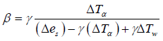
Under the above conditions, Bowen ratio can be calculated from the difference in actual air temperature ΔTα and actual vapor pressure change Δeα over a vertical air column. According to Euser et al. [12]
 (2)
(2)
where ϒ = 0.071khPa °C-1, is the Psychrometric constant for wind speed less than 3.0 m/s. Using measurements from dry and wet surface, temperature and the actual water vaporea Δeα can be calculated using Allen et al. [13]
 (3)
(3)
where; es is the saturation vapor pressure that can be obtained using Allen et al.
 (4)
(4)
Taking measurement at any two reference height 1 and 2 with equations (2) becomes Euser et al.
 (5)
(5)
Equation (5) can be written as;
 (6)
(6)
where each term retains its usual definition. It is observed here that the Bowen Ratio depends only on the Psychometric values of the instrument
With Bowen ration β obtained, the available energy (Rn − G) is partitioned into sensible and latent heat fluxes according to the equations below.
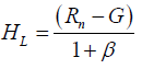 (7)
(7)
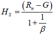 (8)
(8)
where G is the ground heat flux, sometimes represented by HG and Rn is the net radiation flux. Each of the surface energy fluxes is calculated in Wm-2
Aerodynamic Gradient Technique (AGT): One of the widely accepted methods of estimating surface heat fluxes is the Eddy covariance method. The basic foundation of this method rests on the work of Reynold, who came up with decomposition scheme which helps to isolate turbulent component from the mean value of a variable [14].
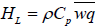
From the covariances only, sensible and latent heat fluxes are estimated using the equations below.
 (9)
(9)
 (10)
(10)
ρ is the air density, Cp is the specific heat capacity of dry air at constant pressure.
ρ = 1.225 kgm-3 Cp= 1004.67 Jkg-1K-1 [15]
However, for profile measurement, the covariances are obtained as shown below
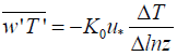 (11)
(11)
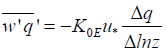 (12)
(12)
where u* is the frictional velocity given by the expression below, K0 and K0E are the eddy diffusivities of heat and water, respectively.
Under stable condition,
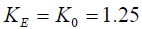 (13)
(13)
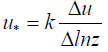 (14)
(14)
Since specific humidity was not measured directly, it can be parameterized from dry and wet bulbs temperatures using equation 15 [16].
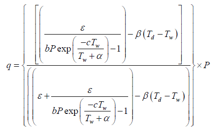 (15)
(15)
where b, c, ε, α and β are constants which are experimentally determined. For general purpose;
b = 1.631kPa-1, c = 17.67 and ε = 0.622g/g, β = 4.0224* 10-4 g)/°C, and α = 243.5°C
Tw = wet bulb temperature, Td = dry bulb temperature, P=ambient pressure and q is the specific humidity
α = 243.5 °C
Aerodynamic with Resistance Technique (ART): Aerodynamic technique deals with the surface diffusivity of matter at the surface layer. Hence, equations (1) and (2) can be expressed in terms of Aerodynamic equations as:
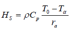 (16)
(16)
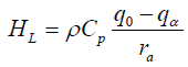 (17)
(17)
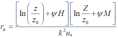
where rα is the aerodynamic resistance. T0 , Tα , q0 and qα are the respective reference surface temperature, air temperature, surface humidity and air humidity.
where k is the Von Kaman constant, θ1 and θ2 are the surface air temperatures at two heights z1 and z2 while u1 and u2 are the respective wind speeds at sea level while ea1 and ea2 are the actual vapor pressure measured at different the same altitudes z1 and z2, respectively.
Where ρ is the air density, Cρ is the specific heat capacity of air at constant pressure, T0 is the surface (skin) temperature, and Tz is the temperature of the air at position z above the surface, q is the specific humidity, rα remains the aerodynamic resistance in sm-1. It is the diffusion resistance to sensible heat transfer between the surface and an altitude z above the surface [17].
 (18)
(18)
 (19)
(19)
but under stable condition [18];
 (20)
(20)
where L is the Obukhov length, z is height, ψM = is the transfer of heat and
ψM = momentum transfer of water.
The aerodynamic method is one of the most widely used indirect methods of computing momentum and sensible heat transfers at the lower surface of the planetary boundary layer. This method only requires atmospheric measurement of input variables at a single altitude alongside with surface properties such as the roughness length as well as the skin temperature (for heat flux). For a very low surface, the equations below are sufficient for computing the fluxes [19-21].
 (21)
(21)
where z is the measurement height, L is the Obukhov length.
Monnin and Obukhov (1954), promulgated, an accepted model for estimating L as given below [14,22]:
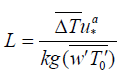 (22)
(22)
where ΔT and  are the variance and the covariance of temperature and wind speed, while g is the acceleration due to gravity, * u is the frictional velocity, k is the von Kaman constant (taken as 0.4) [14].
Results and Discussions
Analysis of all input variables can be obtained from Jegede et al. [10]. However, other needed parameters required for estimation of sensible and latent heat fluxes were parameterized from these meteorological variables. Hence, only the estimated heat fluxes as well as their closure are hereby discussed.
Estimated convective heat fluxes: Figure 2a and b show the daily trend of the estimated sensible and latent heat fluxes from the AG, BR and OBS (Observed from direct measurement by eddy covariance) heat fluxes. It is observed that there was no much difference in the magnitudes of the estimated and measured heat fluxes during the early morning hours. This may be due to the absence of turbulence at such times. However, after sun rise, evolution of turbulence began due to increase intensity of the net solar radiation which triggers other atmospheric parameters into response.
Figure 2: (a-d) Comparative Distribution of Estimated Convective Heat Fluxes for Ile-Ife for day 55: (a) Sensible Heat Flux for Aerodynamic Gradient (AG), Bowen ratio (BR) and Observed (OBS); (b) Latent Heat for (AG), BR and Observed (OBS); (c) Sensible for Aerodynamic (AR) and (OBS); (d) Latent Heat flux for (AR) and (OBS).
From the results, AG yielded a maximum sensible heat flux of 254.37 W/m2 on Julian day 64 at 11:00 LT with a minimum day time value of 12.0 W/m2. Also, mean sensible heat ranges from 0.50 W/m2 to 112.00 W/m2. Latent heat flux has a maximum value of 300.87 W/m2 which is 46.89 W/m2 more than the maximum value of sensible heat flux which is due to the synoptic of the day. The daily mean values range from 10.84 W/m2 to 114.15 W/ m2. Evaluation of estimated heat fluxes with respect to wet day (56), dry day (58) and cloudy day (68) revealed that the mean sensible heat fluxes for the above reference days were 106.24 W/m2, 110.13 W/m2 and 71.83 W/m2, respectively as against the observed values of 143.05 W/m2, 86.69 W/m2 and 85.91 W/m2, respectively for the same set of days. The mean value for wet day is 36.805 W/m2 less than the observed. Hence, AG has under estimated mean flux for the wet day by 36.80 W/m2. This maybe as a result of the fact that sonic anemometer cannot operate properly when it is wet (Jerald, 2002). For latent heat flux, the daytime mean values for the selected synoptic days were respectively 47.97 W/m2, 72.24 W/m2 and 46.46 W/m2 while the observed were 11.40 W/m2, 10.23 W/m2 and 123.08 W/m2, respectively.
The roughness length, z0 was obtained from the plot of lnz against wind speed (u), [14] and was found to be around 0.011 m. The hourly series of the estimated fluxes of sensible and latent heat fluxes are shown in Figures 2 and 3, respectively. In magnitude, Aerodynamic Resistance (AR) scheme performed very poorly for both latent and sensible heat fluxes. The failure of aerodynamic scheme in estimating turbulent fluxes maybe adduced to weak wind speed which is generally a prominent feature of the tropical area [8]. Maximum values of sensible and latent heat fluxes obtained are 1.88 W/m2 which occurred on day 64 of the year at around 12.00 h and 0.38 W/m2 on day 68 around 11:00 h, respectively. The estimations revealed minimum values of -37.05 W/m2 for sensible heat flux at 19:00 h and -36.00 W/m2 for latent heat flux at about the same time. This result has shown that AR is not a good scheme for the theoretical estimation of convictive heat fluxes in the tropics with low wind speed.
Figure 3: (a-d) Comparative Distribution of Estimated Convective Heat Fluxes for Ile-Ife for day 56: (a) Sensible Heat Flux for Aerodynamic Gradient (AG), Bowen ratio (BR) and Observed (OBS); (b) Latent Heat for (AG), BR and Observed (OBS); (c) Sensible Heat Flux for Aerodynamic (AR) and (OBS); (d) Latent Heat Flux for (AR) and (OBS).
The Bowen ratio obtained using equation 3.1 to equation 3.8 was combined with the available energy (RN-G) to obtain the sensible and latent heat fluxes using equation 3.7 and equation 3.8, respectively (Figures 2 and 3). It was observed that during the late night and early morning hours, estimated heat fluxes by BR were fairly constant (00.00 LT – 7.00 LT). Evolution of convective heat began at about 08.00 LT, attained peak values in the late afternoon and descended slowly back to constant values at sunset to late night hours. The maximum day time sensible and latent heat fluxes obtained were 69.36 W/m2 and 469.54 W/m2, respectively. These values were respectively 203.48 W/m2 less and 168.94 W/m2 more than the measured sensible and latent heat fluxes. This proved that BR partitioned the available energy differently into sensible and latent heat fluxes. While latent heat was overestimated, sensible heat flux was underestimated. The day time mean values estimated for sensible and latent heat fluxes were respectively, 41.60 W/m2 and 220.94 W/m2. (Figures 2a-d and 3a-d).
Comparative performance of the calculated values of convective heat flux using different techniques
Figure 4a-c show the scatter plots of the estimated sensible heat fluxes against observed sensible while Figure 4d-f present the scatter plots of the estimated latent heat flux against the observed latent heat flux for day 55 only. For sensible heat flux R2 for BR, AG and AR have mean values of 0.8023, 0.6383 and 0.1045 respectively. Mean values of R for BR, AG and AR are 0.8872, 0.7838 and 0.2968 respectively. The values of R and R2 for AG and BR are good enough for acceptability while those of AR revealed weak correlations. For latent heat flux, the mean values of R2 for BR, AG and AR are 0.6998, 0.4456 and 0.2373 while the corresponding values of R are 0.7873, 0.6261 and 0.4634 respectively. Comparing the values of R for sensible and latent heat fluxes, it was observed that BR and AG estimated sensible heat flux better than latent heat flux while AR estimated poorly for both sensible and latent heat fluxes. It can therefore be established that while AG and BR are good schemes for theoretical estimation of convective heat fluxes, AR is not. However, AG presented better sensible heat flux than BR while BR estimated latent heat flux better than AG. Figure 4a-c.
Figure 4: (a-f) Scatter plots between the Estimated and the Observed Sensible and Latent Heat Fluxes (HS and HL), respectively for Ile-Ife for day 55 using BR, AG and AR.
Energy residuum and closure fraction: In order to further investigate the performances of the schemes, energy residuum was obtained for each of the schemes as well as the measured as the difference between the net radiation flux and the components of the radiation flux (the ground, the latent and the sensible heat fluxes). On the other hand, the closure fraction was obtained as the plot of the available energy to the turbulent fluxes as given by Jerald et al. It was observed that, aerodynamic Resistance technique (AR) has the highest value of residual energy with daily mean ranging from 60.39 W/m2 to 123.26 W/m2. Aerodynamic Gradient (AG) presented daily mean range from -84.19 W/m2 to 93.22 W/m2. Bowen Ratio (BR) daily mean ranges from -5.05 W/m2 to 0.00 W/m2 while the measured (OBS) has daily mean value from -37.62 W/m2 to 52.53 W/m2. The result presented by AR has only positive values, this maybe which is due to the wide range of underestimation. This implies that there was a mixture of overestimations and underestimation. The above results have further proved that AR would not serve as a reliable scheme for theoretical estimation of convective fluxes due to the low wind speed of the research site.
The mean closure fractions for BR, AG, AR and OBS are 99.89 %, 45.94%, 0.41% and 92.88%, respectively. The estimated coefficient of correlations for BR, AG and AR were found to have the following respective ranges; 0.9237 – 0.076, 0.8927 – 0.0678 and 0.3995 – 0.031. However, closure fraction obtained by AG was found to have a better practical agreement with the measured than others. Correlation coefficient and coefficient of determination obtained by each model presented good ranges for BR and AG but were however, very poor for AR.
Summary and Conclusions
The purpose of this research was to identify the most reliable theoretical method of estimating sensible and latent heat fluxes from more routinely atmospheric variables using theoretical approaches. Results obtained from each of the scheme revealed that none of the models performed convincingly good for both sensible and latent heat fluxes. AG yielded a good estimation for sensible heat flux with a percentage difference of about 13.0%. However, AG performed weakly for latent heat flux with a percentage difference of about 53%. The Bowen Ratio Energy Balance Technique presented poor sensible heat flux with a percentage difference of 240% (an under estimation) and latent heat flux with a difference of about 36%. Aerodynamic with resistance Scheme failed for both latent and sensible heat fluxes. From the above percentage difference, it is clear that Bowen Ratio Technique proved more reliable only for latent heat flux while Aerodynamic Gradient is efficient in estimating sensible heat flux. Hence, the two approaches are good for theoretical approach for estimating heat fluxes in the order of performances presented in this research. The need, therefore, for the modification of the Bowen Ratio Technique as literature has it, is a necessity. Aerodynamic with resistance failed altogether for both sensible and latent heat fluxes; which was adduced to the relative poor wind speed or model’s deficiency in application to the site of measurement. Table 1 below shows the summary of the comparing of the estimated (from models) with the measured (Table 1).
| Days |
|
BR |
|
|
|
AG |
|
|
|
AR |
|
|
| |
a(W/m2) |
ß |
R2 |
R |
a(W/m2) |
ß |
R2 |
R |
a(W/m2) |
ß |
R2 |
R |
| 55 |
-2.7495 |
0.1859 |
0.6193 |
0.787 |
10.144 |
0.3778 |
0.7507 |
0.8664 |
0.0006 |
-0.0002 |
0.0175 |
0.1323 |
| 56 |
-61,553 |
0.1385 |
0.6686 |
0.8177 |
3.6045 |
0.7744 |
0.7502 |
0.8661 |
-0.0126 |
0.0107 |
0.3795 |
0.616 |
| 58 |
6.7986 |
0.1198 |
0.2764 |
0.5257 |
1.3294 |
1.0748 |
0.4056 |
0.6369 |
0.3583 |
-0.0019 |
0.1224 |
0.3499 |
| 59 |
2.8345 |
0.2119 |
0.9338 |
0.9663 |
9.2062 |
0.2082 |
0.4544 |
0.6741 |
-0.1505 |
0.0009 |
0.014 |
0.1183 |
| 60 |
5.8313 |
0.189 |
0.864 |
0.9295 |
1.3294 |
1.0748 |
0.4056 |
0.6369 |
0.3583 |
-0.0019 |
0.1224 |
0.3499 |
| 61 |
1.4876 |
0.3064 |
0.9746 |
0.9872 |
0.2375 |
0.6277 |
0.8081 |
0.8989 |
-0.0628 |
0.0015 |
0.1763 |
0.4199 |
| 62 |
0.4524 |
0.2939 |
0.9836 |
0.9918 |
13.531 |
0.8074 |
0.8607 |
0.9277 |
-0.0303 |
0.0005 |
0.0773 |
0.278 |
| 63 |
7.7883 |
0.3133 |
0.879 |
0.9376 |
14.297 |
0.8231 |
0.6405 |
0.8003 |
-1.3969 |
0.0163 |
0.0674 |
0.2596 |
| 64 |
3.1606 |
0.3116 |
0.753 |
0.8678 |
-4.6389 |
1.6639 |
0.8033 |
0.8963 |
-0.7616 |
0.0178 |
0.1211 |
0.348 |
| 65 |
6.6181 |
0.4175 |
0.9532 |
0.9763 |
4.0217 |
2.0293 |
0.8872 |
0.9419 |
-0.8395 |
0.0193 |
0.0623 |
0.2496 |
| 66 |
5.6644 |
0.4167 |
0.8754 |
0.9356 |
-30.493 |
2.3782 |
0.8563 |
0.9254 |
-0.9836 |
0.0212 |
0.1089 |
0.33 |
| 67 |
6.7959 |
0.4547 |
0.9336 |
0.9662 |
-64.683 |
1.4414 |
0.5154 |
0.717914 |
-4.2825 |
0.0376 |
0.0705 |
0.2655 |
| 68 |
0.0384 |
0.5336 |
0.7137 |
0.8448 |
0.9047 |
0.0065 |
0.1602 |
0.40025 |
-4.1016 |
0.0258 |
0.0199 |
0.1411 |
Table 1: Correlation parameters from the comparison of estimated with measured sensible heat fluxes for Ile-Ife; where a is the value of the estimated heat flux corresponding to the least value of the measured flux, ß is the Gradient, R2 is the coefficient of determination and R is the correlation coefficient.
Acknowledgement
The authors sincerely appreciate Prof. O. O. Jegede from the Department of Physics, Obafemi Awolowo University, Ile- Ife, Nigeria, and Prof. A. A. Balogun from the Department of Meteorology, Federal University of Technology, Akure, Nigeria, for their salient contributions.
References
- Carlos J, Catherine P, Filine A (2009) Toward an estimation of global land surface heat fluxes from multisatellite observations. J Geophys Res 114: D06305.
- Grimmond CSB, Oke TR (2002) Turbulent heat in urban areas: Observations and a Local-Scale Urban Meteorological Parameterization Scheme (LUMPS). J Applied Meteorology 41: 1-7.
- Katavoutas G, Flocas HA, Tsitsomitsiou (2014) Thermal comfort in hot outdoor environment under unsteady conditions. Advances in Meteorology, Climate and Atmospheric Physics, Greece, 2: 195-200.
- Jegede OO (1997) Fluxes of sensible in the surface layer estimated from the profile measurements of wind and temperature at a tropical station. Atmosfera 10: 213-223.
- Balogun AA, Foken Th, Jegede OO, Olaleye JO (2002a) Estimation of sensible and latent heat fluxes over bare soil using Bowen ratio energy balance method at humid tropical site. J Afri Meteorol Sci 5: 63-71.
- Balogun AA, Jegede OO, Foken Th, Olaleye JO (2002b) Comparison of two Bowen ratio methods for estimating sensible and latent heat fluxes at Ile-Ife. J African Meteorol Soc 5: 63-69.
- Ohmura A (1982) Object criteria for rejecting data for Bowen Ratio flux calculations. J Appl Meteorol 31: 595-598.
- Omokungbe OR, Ayoola MA, Jegede OO (2012) Diurnal characteristics of the surface energy fluxes at a tropical site in Ile-Ife, Nigeria. Ife J Science: 14: 195-206.
- Jerald AB, Kenneth CC (2002) Examination of the surface energy budget: A Comparison of Eddy-Correlation and Bowen Ratio Measurement System. J Hydrometeorol 4: 160.
- Jegede OO, Mauder M, Okobgue EC, Foken T, Balogun EE, et al. (2004) The Nigeria Meteorological Experiment (NIMEX-1): An Overview. Ife J Science 6: 191-202.
- Todd RW, Evett SR, Howell TA (2000) The Bowen ratio-energy balance method for estimating latent heat flux of irrigated alfalfa evaluated in a semi-arid environment. Agric Forest Meteorol 103: 335-348.
- Euser T, Luxemburg WMJ, Everson CS, Mengistu MG, Clulow AD, et al. (2014) A new method to measure Bowen ratios using high-resolution vertical dry and wet bulb temperature profiles. J Hydrol Earth Syst Sci 18: 2021-2032.
- Allen RG, Jensen ME, Wright JL, Burman RD (1989) Operational estimates of reference evapotranspiration. Agron J 81: 650-662.
- Arya P (2001) Introduction to Micrometeorology. 2nd edition, Academic Press, USA, 79: 11-13.
- Glickman TS (2000) Glosssary of Meteorology. Am Meteorol Soc, Boston, MA, USA.
- Stull RB (2000) Meteorology for Scientist and Engineers. 2nd Edition, United States.
- Kalma JG (1989) A Comparison of expression for the aerodynamic resistance to sensible heat transfer. CSIRO Division of Water Resources Technical Memorandum, 89/6, pp: 11.
- Charnock H (1955) Wind stress on water surface. Quart J Roy Meteorol Soc 81: 639-642.
- Webb EK (1970) Profile Relationship: The –Linear Range, and Extension to Strong Stability. QJ Meteorol Soc 96: 67-90.
- Businger JA, Wyngaard JC, Izumi Y, Bradley EF (1971) Flux profile relationships in atmospheric surface layer. J Atmos Sci 28: 181-189.
- Oladosu OR, Jegede OO, Sunmonu LA, Adediji AT (2007) Bowen ratio estimation of surface energy fluxes in a humid tropical agricultural site, Ile-If, Nigeria. Indian J Radio and Space Physics 36: 213-218.
- Monin AS, Obukhov AM (1954) Basic laws of turbulence mixing in the atmosphere near the ground. Tr Akad Nauk SSSR Geofiz Inst.