Research Article - (2025) Volume 9, Issue 1
Mathematical Modelling of Bovine Tuberculosis Transmission Dynamics: Role of Combination of Control Measure
Sylas Oswald1*,
Theresia Crispin Marijani1,
Goodluck Mika Mlay1 and
Winifrida Benedict Kidima2
1Department of Mathematics, University of Dar-es-Salaam, P.O.Box 35062, Dar-es-salaam, Tanzania
2Department of Zoology and Wildlife Conservation, University of Dar-es-Salaam, P.O.Box 35064, Dar-es-salaam, Tanzania
*Correspondence:
Sylas Oswald, Department of Mathematics, University of Dar-es-Salaam, P.O.Box 35062, Dar-es-salaam,
Tanzania,
Email:
Received: 12-Jun-2024, Manuscript No. IPJVMS-24-20424;
Editor assigned: 14-Jun-2024, Pre QC No. IPJVMS-24-20424 (PQ);
Reviewed: 28-Jun-2024, QC No. IPJVMS-24-20424;
Revised: 12-Mar-2025, Manuscript No. IPJVMS-24-20424 (R);
Published:
19-Mar-2025, DOI: 10.36648/2574-2868.9.1.41
Abstract
Bovine Tuberculosis (BTB) is a contagious and potentially life-threatening infectious disease of cattle caused by Mycobacterium bovis (M. bovis) that lives in various environment depending on prevailing weather conditions (Temperature and humidity). Globally, the BTB is one of the diseases with utmost public health challenges which places economic and financial burdens on the society. To curb the disease, a mathematical model for the spread of BTB among human and cattle populations including preventive measures was formulated. The model analysis focused on the existence of disease-free and endemic equilibria points and their stabilities. The study used normalized forward sensitivity index method to analyze the model, and results revealed that the most sensitive parameter is the contaminated environment or inter-cattle transmission. Moreover, the study determined the best way of curbing the spread of BTB disease in the human and cattle populations using three interventions: public health education campaign, treatment and vaccination. Subsequently, the study performed numerical simulations whose results affirm the positive effects of a combination of control measures on the magnitude of infections among human and cattle population.
Keywords
Mycobacterium bovis; Bovine Tuberculosis (BTB), Spectral radius; Most sensitive; Bifurcation coefficients; Stability analysis; Runge-Kutta fourth (RK4) order
Introduction
Bovine Tuberculosis (BTB) is a contagious and life-threatening infectious disease of cattle. The bacterium Mycobacterium bovis (M. bovis) that causes disease, can also afflict many other mammals such as humans, goats, pigs, cats and dogs. BTB remains a significant challenge in both human and animal health worldwide. It poses a substantial economic burden, particularly in regions heavily reliant on live-stock agriculture. In 1993, the disease was declared a global state of emergency. Despite our knowledge of how to effectively prevent and cure BTB through half a century of development and progress, more than 1.6 million people have still died from it. In 2014, BTB claimed the lives of 1.5 million people, including 890,000 men, 480,000 women, and 140,000 children. India, Indonesia, and China had the largest number of cases, accounting for 23%, 10%, and 10% of the global total, respectively. Traditional control measures, such as culling infected animals and movement restrictions, have had limited success in curbing the transmission of BTB. To address this complex issue, researchers have increasingly turned to mathematical modelling to gain insights into the dynamics of BTB transmission and assess the potential impact of various control strategies. This study delves into the mathematical modelling of BTB transmission dynamics, with a novel focus on the synergistic role of a combination of vaccination, treatment, and education campaigns as control measures [1].
The transmission route entails direct, close contact through inhaling sputum droplets (thick mucus produced in the lungs) contaminated with M. bovis bacteria exhaled by infected animals. On the other hand, indirect transmission of the disease can occur when one comes into contact with an infected animal or ingests material heavily contaminated with M. bovis, such as sputum, pus, urine, feces, and other excrement of infected animals. There are inherent practical difficulties associated with detecting M. bovis in environmental samples. However, the bacteria have been traced in diverse sources, such as soil, excrement, hay, and pasture.
Bovine Tuberculosis: A Global Challenge
Bovine tuberculosis poses a substantial threat to both animal and human populations. In cattle, it results in reduced milk and meat production, increased slaughterhouse condemnation rates, and trade restrictions, contributing significantly to economic losses in affected regions. In humans, zoonotic transmission of BTB remains a concern, particularly in areas where close contact with infected cattle occurs. Given its impact on both public health and the livestock industry, BTB demands innovative and effective control measures [2-5].
Mathematical Modelling in Infectious Disease Control
Mathematical modelling has proven to be a powerful tool in understanding and predicting the dynamics of infectious diseases. In the context of BTB, previous studies have employed compartmental models, network models, and agent-based models to simulate disease spread and evaluate control strategies. These models have provided valuable insights into the role of factors such as cattle demographics, wildlife reservoirs, and testing protocols in BTB transmission dynamics.
Individual Control Measures
Many studies have assessed the efficacy of individual control measures, such as vaccination and antimi-crobial treatment, in reducing BTB prevalence. Vaccination with Bacillus Calmette-Gu´erin (BCG) has shown promise in reducing the severity of BTB in cattle. Antimicrobial treatment can help clear infections but is often logistically challenging due to the lengthy treatment duration and concerns about antibiotic resistance.
Materials and Methods
Education Campaigns as a Control Measure
Education campaigns aimed at promoting best practices in cattle management, biosecurity measures, and early disease detection have been recognized as crucial components of BTB control. These campaigns empower farmers and stakeholders with knowledge to reduce the risk of BTB transmission within and between herds.
In Africa and Europe, bovine tuberculosis is a serious threat to the economy as well as human and animal health. For example, presented a deterministic model for examining the impact of separating two large human populations based on the probability of coming into contact with cattle for the prevention of bovine tuberculosis. The model encompasses three types of incidents: Those occurring between cattle, between humans, and between cattle and humans. The results of the study, based on the stability of the disease-free equilibrium and sensitivity analysis of the model’s parameters, showed that quarantine measures for cattle and the parameter related to medical masks significantly contributed to reducing the basic reproduction number and, consequently, decreasing the disease transmission rate. The effects of vaccines on cattle, treatments, public health education campaigns for humans, and communal water source sharing, in relation to disease transmission, were not fully considered.
The study by also presented a dynamic mathematical model for the transmission of bovine BTB. The results from the model simulations supported vaccine administration as the best strategy for reducing BTB infections. Furthermore, they suggested that coupling a public health education campaign with treatment for humans could maintain R0 below one, significantly reducing the spread of bovine tuberculosis. However, their study did not address the impact of treatment as a measure for controlling the transmission dynamics of bovine tuberculosis.
A study by revealed that the use of slaughter and quarantine methods to reduce the number of infectious cattle was found to be the most important control measures to minimize the prevalence of BTB disease.
The study done by revealed that a relatively high proportion of BTB infections in the Ngorongoro district are due to the husbandry practices of a semi-nomadic system where the Maasai search for water and pasture during the dry season. It is recommended that implementing an education campaign for cattle owners would be the best solution.
In developing countries such as Tanzania, Bovine Tuberculosis (BTB) remains a serious threat to human health because the disease is still largely hidden in society. Reported cases of BTB in Tanzania are concentrated in specific regions, including the Northern part of the country (Arusha, Kilimanjaro, and Manyara), dairy farms in Kibaha, and some areas in Morogoro districts. The prevalence of the disease varies from one region to another, depending on the concentration of cattle herds in a particular place, ranging from 0.2 percent to 13.3 percent.
Novelty of the Study
While previous research has explored individual control measures in isolation, this study stands out for its innovative approach in combining vaccination, treatment, and education campaigns within a mathematical modelling framework. Investigating the synergistic effects of these measures can provide a more comprehensive understanding of their potential impact on BTB transmission dynamics. Moreover, it addresses the practical question of how these measures can be integrated into a cohesive control strategy to reduce both the prevalence of BTB and its economic burden [6-10].
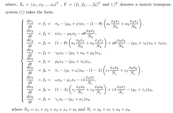
Model Formulation
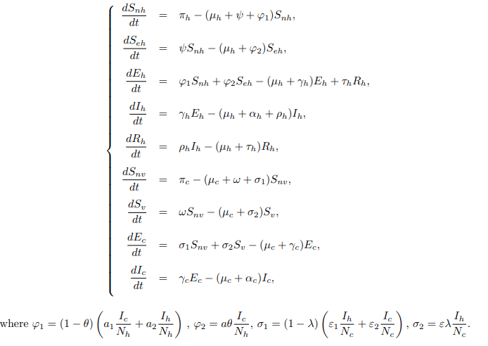
The model under consideration here entails two populations: humans and cattle, which often come into contact. The management system for grazing is a ranching system in which only cattle are confined. The model operates on the assumption that at any time t, the human population, denoted by Nh(t), is divided into five classes: Susceptible noneducated (Snh(t)), Susceptible educated (Seh(t)), Exposed (Eh(t)), Infectious (Ih(t)), and Recovered (Rh(t)) individuals.
The total human population Nh(t) is given by Nh(t)=Snh(t)+ Seh(t)+Eh(t)+Ih(t)+Rh(t).
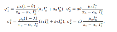
The recruitment of humans into the susceptible non-educated class occurs at a constant rate πh. The assumption is that the education strategy is executed at a rate of ψ only for susceptible, non-educated humans to reduce the disease’s transmissibility. Moreover, the study assumes that the education given to a targeted group does not necessarily guarantee lifelong protection. Susceptible non-educated humans can acquire infection through the consumption of cattle products and aerosols from infected cattle, as well as through inter-human transmission at the rate φ1, and then move to the exposed class. The variable φ1 is the force of infection given by

where a1 and a2 are probabilities that infectious cattle and human infects susceptible non educated humans, respectively and θ ∈ [0, 1] is the efficacy of the education campaign that is being implemented. Furthermore, an educated human may contract the disease by consuming contaminated cattle products and inhaling aerosols from infected cattle at the rate φ2, leading to a transition to the exposed class. The variable φ2 represents the force of infection for susceptible educated humans.
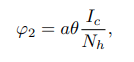
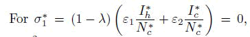
where a is the probability that infectious cattle infects susceptible educated human. If no education campaign is extended to susceptible non-educated human, then θ=0. Both educated and non-educated susceptible humans may leave their respective classes following the occurrence of natural death at a rate of μh. Some of the exposed individuals leave the compartment upon gaining full recovery, denoted as ρh, due to treatment and a natural or disease-induced death rate of μh and αh, respectively. Considering the transmission dynamics of BTB disease, the study assumes that the treatment does not guarantee permanent protection. As such, recovered humans may either progress to the exposed class at a rate of τh or leave the compartment following the occurrence of natural death at a rate of μh. This study presupposes that at any time t, the cattle population denoted by Nc(t) is divided into four classes, of Susceptible nonvaccinated Snv(t), Susceptible vaccinated Sv(t), Exposed Ec(t) and Infectious Ic(t) cattle. The total cattle population Nc(t) is given by Nc(t)=Snc(t)+Sv(t)+Ec(t)+Ic(t). At any given time t, it is also presumed that cattle are recruited into the nonvaccinated cattle group at a constant rate πc. Healthier cattle are vaccinated at a rate ω to reduce the transmission of M. bovis from the contaminated environment and inter-cattle transmission. Susceptible non-vaccinated cattle can contract infections from their respective environment, inter-cattle transmission, and infection from infected humans. The progression to the exposed class occurs at a rate σ1. The variable σ1 represents the force of infection for nonvaccinated cattle.
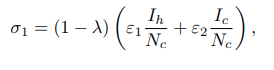
Where ε1 is the probability of an infected human infecting susceptible, non-vaccinated cattle. Moreover, the presumption is that it is difficult to differentiate infected cattle from a contaminated environment or from inter-cattle transmission. ε2 is the rate at which cattle get infected through nose-to-nose contact, aerosol inhalation, grazing areas, and all other environmental elements that can infect cattle. λ ∈ [0, 1] represents the vaccine efficacy. If no susceptible cattle are vaccinated, then λ=0. Furthermore, vaccinated cattle may contract infection from both a contaminated environment and inter-cattle transmission at the rate σ2, leading them to move to the exposed class. The variable σ2 constitutes the force of infection for susceptible vaccinated cattle, as given by
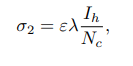
Where ε represents the probability that an infected human will transmit the disease to susceptible vaccinated cattle. Both vaccinated and non-vaccinated susceptibles may leave their respective classes due to natural death at a rate of μc. Exposed cattle also exit this class, either because of natural death 5 at a rate of μc or due to progressive incubation into the infectious class at a rate of γc. Furthermore, infected cattle exit the class through natural death at a rate of μc and disease-induced death at a rate of αc (Figure 1).
Model Diagram

Figure 1: Schematic flow diagram for the dynamics of bovine tuberculosis disease in the presence of some intervention strategies for model.
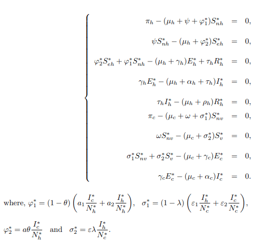
Model Equations
The biological description and schematic flow diagram in Figure 1 together result in the following system of nine nonlinear ordinary differential equations (Table 1).
| Parameter |
Description |
Values |
| πh |
Human recruitment rate |
36 |
| πc |
Cattle recruitment rate |
200 |
| a1 |
Probability that infectious cattle infects susceptible non-educated human |
0.55 |
| a2 |
Contaminated environment/inter-human transmission |
0.35 |
| a |
Probability that an infectious cattle infect a susceptible educated human |
0.000010995 |
| ε1 |
Probability that an infectious human infects a susceptible cattle |
0.000057803 |
| ε2 |
Contaminated environment/inter-cattle transmission |
0.908 |
| ε |
Probability that an infected human infects a susceptible vaccinated cattle |
0.000016252 |
| ρh |
Human recovery rate with treatment |
0.098 |
| τh |
Removal rate to latent state |
0.01 |
| γh |
Progression rate to infectious state |
0.18 |
| γc |
Progression rate to infectious state |
0.18 |
| µh |
Human natural death rate |
0.0023 |
| µc |
Cattle natural death rate |
0.013 |
| αh |
Human death rate due to disease |
0.139 |
| αc |
Cattle death rate due to disease |
0.12 |
| θ |
Education efficacy |
0.75 |
| λ |
Vaccine efficacy |
0.25 |
| Ψ |
Per capita education rate |
0.85 |
| ω |
Per capita vaccination rate |
0.67 |
Table 1: Parameters and their descriptions.
Basic Properties of the Model
Positivity of the solutions: To ensure that the model (1) is epidemiologically meaningful and well-posed, it is necessary to demonstrate that all state variables are non-negative ∀t ≥ 0.
Lemma 1. Let {Snh(0) ≥ 0, Seh(0) ≥ 0, Eh(0) ≥ 0, Ih(0) ≥ 0, Rh(0) ≥ 0, Snv(0) ≥ 0, Sv(0) ≥ 0, Ec(0) ≥ 0 and Ic(0) ≥ 0 } of themodel system (1) are satisfied then the solutions {Snh, Seh, Eh, Ih, Rh, Snv, Sv, Ec, Ic } are non-negative for all t ≥ 0 in Ω.
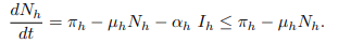
Proof. From the first equation of system (1),
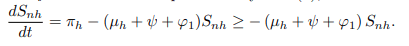
In the absence of human recruitment πh it follows that
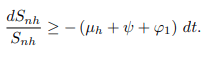
Upon integration gives,
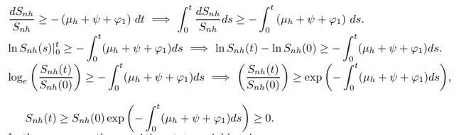
In the same way, the remaining state variables give;
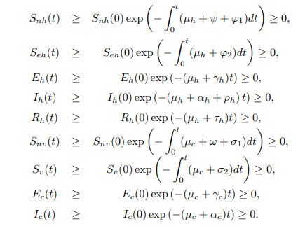
Therefore, the solution set {Snh, Seh, Eh, Ih, Rh, Snv, Sv, Ec, Ic} of the model system (1) is non negative for all t ≥ 0 in Ω.
Invariant Region
Lemma 2. The feasible region defined by Ω=Ωh ∪ Ωc ∈ R5 + × R4 + where Ωh={Snh, Seh, Eh, Ih, Rh ∈ R5 +: Snh+Seh+Eh+Ih+Rh=Nh ≤ πh/μh} and Ωc = {Snv, Sv, Ec, Ic ∈ R4 +:Snv+Sv+Ec+Ic=Nc ≤ πc/μc}, is positively invariant and attracting with regard to the model system (1).
Proof. Given Snh (0) ≥ 0, Seh (0) ≥ 0, Eh (0) ≥ 0, Ih (0) ≥ 0, Rh (0) ≥ 0, Snv (0) ≥ 0, vs. (0) ≥ 0, Ec (0) ≥ 0 and Ic (0) ≥ 0, it is sufficient to prove that {Snh(t), Seh(t), Eh(t), Ih(t), Rh(t), Snv(t), Sv(t), Ec(t), Ic(t)} ∈ R9+ is bounded.
Case 1: By summing equations for human population from model system gives;
Separating variables and applying anti-derivative of an integrating factor it gives;
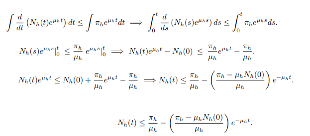
The same procedure can be used to prove that;
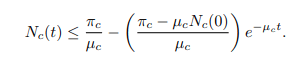
Since the total population Nh(t) as well as Nc(t) is positive for all t ≥ 0. It is well defined that,
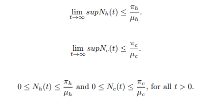
This proves that all solutions of the BTB model system (1) with initial conditions in Ω for all t>0.
Model Analysis
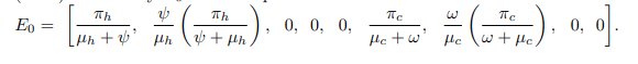
Disease free equilibrium: Disease-Free Equilibrium (DFE) of the mathematical model system (1) is the point where there is no disease. Disease-free equilibrium point is obtained by setting Eh=Ih=Rh=Ec=Ic=0 in all equations. Now, Let E0 be disease-free equilibrium point. Therefore, the Disease Free Equilibrium Point (DFE) denoted by E0 can be expressed as
The Effective Reproduction Number
The Effective Reproduction Number (Re) is the expected number of secondary cases produced by a single (typical) infection in a completely susceptible population and in nonsusceptible hosts [6,7,10]. Effective reproduction number (Re) is the the spectral radius of the next-generation matrix, denoted 10 by Re=ρ(FV−1) at DFE with F and V, respectively given by
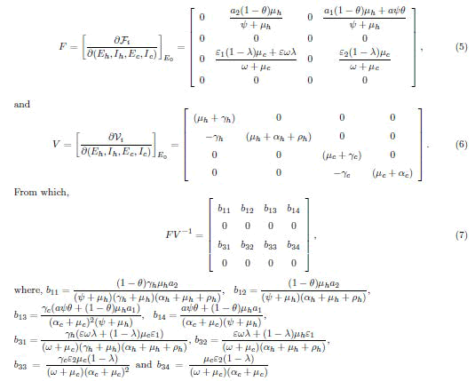
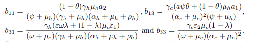
It follows that the effective reproduction number of the model system (1), is given by
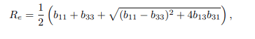
such that,
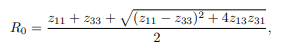
So, when there is no intervention strategy such that ψ=0 and ω=0,” which refers to the education campaign and vaccination rate,” and without any treatment for individual humans being implemented (ρh=0), then the basic reproduction number R0 will be
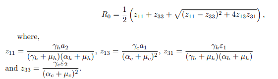
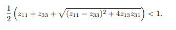
Biologically, it is meaningful to compare the threshold values: the basic reproduction number without a vaccine, denoted as R0, and the effective reproduction numbers with and without a vaccine, denoted as Rv and Re respectively, such that Rev0. The basic reproduction number, often denoted as R0, plays a crucial role in epidemiological studies by facilitating predictions of future infections of interest. When the basic reproduction number is less than one (R0<1), it implies that, on average, an infectious individual leads to the infection of fewer than one other individual. Consequently, over time, the bTB disease could naturally die out, leading to a population free from BTB. In other words, both the human and cattle populations would remain free from the disease invasion if R0<1 [11-15]
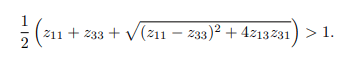
Conversely, if the basic reproduction number (R0) is greater than one, it implies that each infected individual, on average, will lead to more than one newly infected individual. In this scenario, the infection persists, causing the disease to continue spreading in the population. Therefore, if R0>1, BTB will continue to spread
Local Stability of Disease-Free Equilibrium (DFE)
The local stability analysis of DFE enables us to understand how a system behaves near an equilibrium point, but not necessarily at a specific equilibrium point. In other words, local stability investigates the nature of the system in the vicinity of the equilibrium point.
Theorem 3.1. The BTB model system at DFE (E0) is locally asymptotically stable if Re<1 and unstable if Re>1.
Proof. The Jacobian matrix of the model system at disease free equilibrium point (E0) is given by
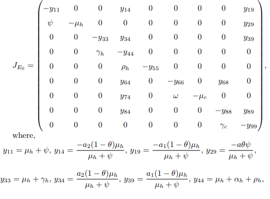
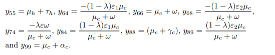
From the Jacobian matrix JE0, the first, fifth and seventh columns contains diagonal entries. Therefore, the diagonals −μh, −(μh + τh), and −μc are the three eigenvalues of the Jacobian JE0. Thus, excluding these columns and the corresponding rows, the remaining eigenvalues are computed. Then the reduced 6 × 6 matrix from JE0 becomes.
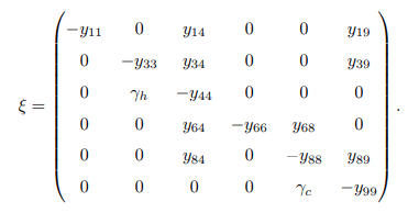
From the Jacobian matrix ξ, the first and fourth columns contains diagonal entries. Therefore, the diagonals − (μh + ψ) and − (μc + ω) are the two eigenvalues of the Jacobian ξ. Thus, excluding these columns and the corresponding rows, the remaining eigenvalues are computed. Then the reduced 4 × 4 matrix from ξ bec becomes.
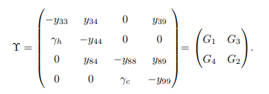
Matrices G1, G2, G3 and G4 are defined as follows
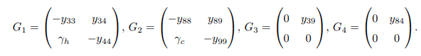
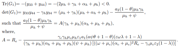
Apparently, matrices G3 and G4 are singular matrices with | G3| = 0 and |G4| = 0. Now, it is sufficient to demonstrate that the disease-free equilibrium point of the model system (1) is stable only when the trace and determinant of matrices G1 and G2 are negative and positive, respectively. Trace and determinant of matrix G1 denoted by Tr(G1) and det(G1) are respectively given by.
Trace and determinant of matrix G2 denoted by Tr(G2) and det(G2) are respectively given by
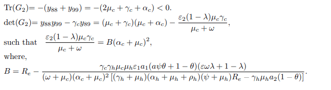
Thus det(G1)> 0 and det(G2)> 0 if and only if Re<1. Since the traces of matrix G1 and G2 are negative and the determinants are strictly greater than zero when Re<1, then the disease-free equilibrium point E0 is locally asymptotically stable when Re<1 and unstable otherwise. Epidemiologically, it implies that the bTB disease can be eliminated in the endemic area when Re<1, particularly when the vaccination rate (ω) is kept constant without limitation, and the education campaign rate (ψ) is also executed for every individual. Conversely, if Re>1, then each infectious individual produces more than one new infected individual, implying that the disease can spread rapidly in the entire population [16-20].
Global Stability of Disease-Free Equilibrium (DFE)
This subsection analyses the global stability pertaining to DFE aimed to establish the asymptotic behaviour of the model system (1) beyond just the neighbourhood points of the model disease-free steady state.
Lemma 3. The disease-free equilibrium point is globally asymptotically stable if Re<1 and unstable if Re>1.
Proof. The approach of [6] is used to analyse the global stability of DFE of the model system (1). Using this approach, the model system (1) is written as follows.
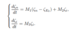
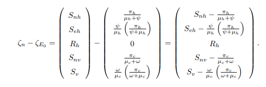
where ζn stands for classes that do not transmit bTB disease, that is ζn=(Snh, Seh, Rh, Snv, Sv) T and ζi stands for classes that can transmit bTB disease, that is ζi=(Ih, Eh, Ec, Ic) T. Here, T stands for the transposition of ζn and ζi, and also ζE0 is ζn at DFE (E0). The matrix M1 is obtained by differentiating the nontransmitting equations of the model system (1) with respect to non-transmitting variables at E0, whereas the matrix M2 is obtained by differentiating the non-transmitting equations of the model system (1) with respect to the transmitting variables. The disease-free equilibrium point (E0) is globally asymptotically stable if the eigenvalues of M1 are real and negative, and if M3 is a Metzler stable matrix with nonnegative off-diagonal elements. Therefore, the model system (1) yields the following.
Also,
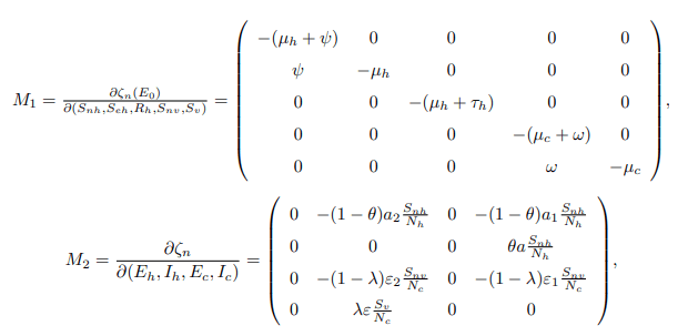
Since the matrix M1 is a lower triangular matrix, then the eigenvalues will be the diagonal entries presented as follows: ξ1=−(μh+ψ), ξ2=−μh, ξ3=−(μc+ω) and ξ4=−μc which are all negative and real. This shows that at the DFE the system dζn/dt=M1(ζn−ζE0)+M2ζi is globally asymptotically stable. Furthermore, the matrix M3 is obtained by differentiating the transmitting equations of the model system (1) with respect to the transmitting variables which gives

Testing whether the matrix M3 is a Metzler stable matrix requires applying the approach as propounded by [16,11]. The following Lemma is used.
Lemma 4. Let G be a square Metzler matrix stable which can be written in block form
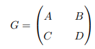
where A and D are square matrices. Then, G is a Metzler stable matrix if and only if matrix A and D−CA−1B or matrix D and A−BD−1C are Metzler stable.
By comparing the matrix M3 and a square Metzler matrix G, then the matrices A, B, C and D are expressed as follows:
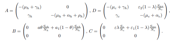
After some computations and simplifications,
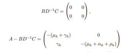
A − BD−1C is said to be Metzler stable matrix if and only if (μh +γh) (μh+αh+ρh) ≥ 0. As already noted, it can be seen that matrix M1 has all the eigenvalues that are real and negative and matrix M3 is the Metzler matrix as its off-diagonal elements are so non-negative, that |A−BD−1C| ≥ 0 =⇒ M3(i,j) ≥ 0 for all indices i/=j. Implicitly, that the disease-free equilibrium point is globally asymptotically stable when Re<1, otherwise it is unstable. In biological terms, the bTB disease will eventually die out in the population given Re<1 no matter how huge the disease invaded. Otherwise, if Re>1 the disease will spread even more as there will be many new infections in the population.
Endemic Equilibrium Point (EEP)
Existence of the equilibrium solutions: The Endemic Equilibrium (EE) denoted by E∗ such that E∗=(S∗nh, S∗eh, E∗h, I∗h, R∗h, S∗nv, S∗v, E∗c, I∗c) is the state where the population is not free from the infection. At this point the disease persists in the population. In other words, the disease cannot be eradicated from the population. In the case of bTB, the number of infectious cases is not equal to zero such that, Eh/=0, Ih/=0, Rh/=0, Ec/=0, Ic/=0. Setting each equation in the model system (1) equal to zero, then the steady state of the system becomes.
Finally, when solving for the corresponding variable from equation (11) the Endemic Equilibrium denoted by E∗=(S∗nh, S∗eh, E∗h, I∗h, R∗h, S∗nv, S∗v, E∗c, I∗c) is solved and given by
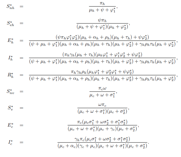
where,

From equation (12), the value of I∗h and I∗c is substituted into
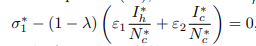
and after some algebraic computations and simplifications, a polynomial of degree three results Aσ1 ∗3+Bσ1 ∗2+Cσ1 ∗=0. Upon algebraic simplification, Aσ1 ∗3+Bσ1 ∗2+Cσ1 ∗=0 results to σ1 ∗∗Aσ1 ∗2+Bσ∗ 1+C=0, where σ1 ∗=0 or Aσ1 ∗2+Bσ∗ 1+C=0
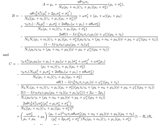
corresponds to Disease Free Equilibrium (DFE), whereas Aσ1 ∗2 +Bσ∗1+C=0, can also be written in the form:
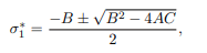
which satisfies Endemic Equilibrium. The value of A is strictly positive. Depending on the signs of B and C, there are three cases to consider as having positive real root of the force of infection (σ∗1) as follows:
Case 1: If B<0 then model system (1) has a stable endemic equilibrium point when C<0. This equilibrium happens when Re>1 as interpreted from (13). In this case backward bifurcation is not possible due to the absence of multiple equilibria.
Case 2: Exactly one endemic equilibrium point. Suppose B<0 and C=0 or B2−4AC=0. In other words, the polynomial Aσ1 ∗2 +Bσ∗ 1+C=0 has just one positive root and hence the model system (1) has unique endemic equilibrium point.
Case 3: Two endemic equilibria. If B<0, C>0 and B2−4AC>0, then the polynomial Aσ1 ∗2+Bσ∗ 1+C=0 has two positive real roots. In other words, the model system (1) has two endemic equilibria and hence there is a possibility of backward bifurcation. These three cases are summarized under theorem 3.2.
Theorem 3.2. The number of positive endemic equilibria of bovine tuberculosis model (1) is hereunder summarised thus:
If C<0, Re>1, then the system has a unique endemic equilibrium.
If B<0 and C=0 or B2−4AC=0, then the system has exactly one endemic equilibrium.
If B<0, C>0 and B2−4AC>0, then the system has exactly two endemic equilibria.
Otherwise there are no endemic equilibria, i.e., when AC>0 and B>0.
Stability of Endemic Equilibrium Point (EEP) of Model with Interventions
In epidemiological models, forward or backward bifurcation has vital implications for the biological control measures of infectious diseases. Bifurcation analysis of the equilibrium points reveals whether the disease is completely reducible or persistent in the afflicted population. This analysis occurs at the disease-free equilibrium using Center Manifold theory, as presented in [6]. It is done by renaming the state variables of the model system as follows.

Resulting system can be written in the form of
Let ε∗2 be the bifurcation parameter, then, the system is a system of model equations at disease free equilibrium point when ε2=ε∗2 with R0=1. Hence, solving for ε∗2 from R0=1 in
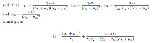
Next, the system is transformed with ε2=ε∗2, which possesses a simple zero eigenvalue. Center Manifold Theory is employed to analyze the dynamics of in the vicinity of ε2=ε∗2. Consequently, the Jacobian matrix of the system at the disease-free equilibrium, denoted as J (ε∗2), is given by
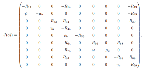

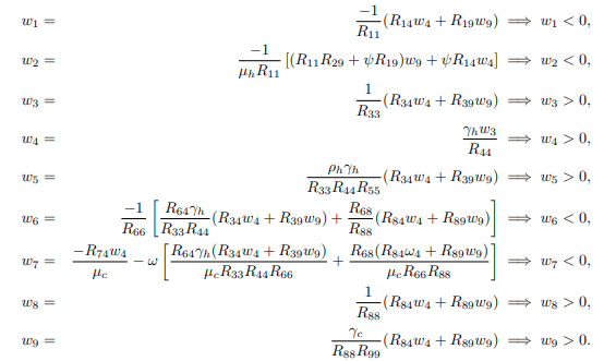
Now, the right and left eigenvectors associated with the zero eigenvalues are calculated. The right eigenvector associated with the zero eigenvalue is given by w=(w1, w2, ..., w9)T, which results in the following equations:
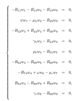
Solving the system (15) for wi′s, i=1, 2, ..., 9, gives the following right eigenvectors
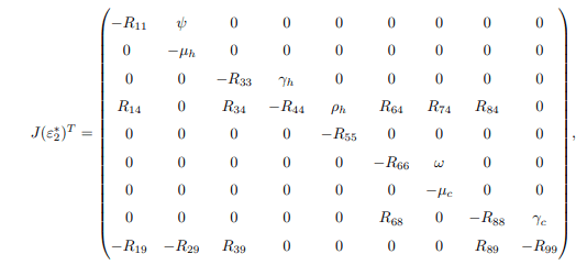
furthermore, to calculate left eigenvector given by v=(v1, v2, ..., v9)T, which satisfy v. w=1, the matrix J(ε∗2) is transposed and becomes.
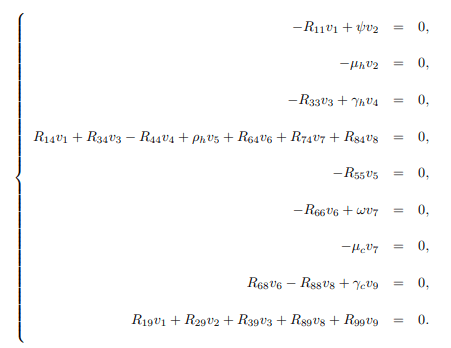
Then solving J(ε∗2)T, the following are obtained
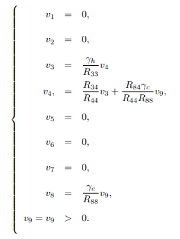
Solving the system (16) for vi's, i = 1, 2, ..., 9, yields the following left eigenvectors
From [6], Theorem 4:1 is used to establish the conditions for the existence of forward or backward bifurcations of the endemic equilibrium point near R0=1.
Lemma 5. Consider the following general system of ordinary differential equations with a parameter β such that
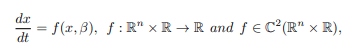
such that f (0, β) ≡ 0, where 0 is an equilibrium point of the system with the following conditions:
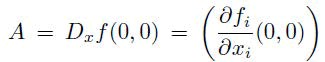
is the linearization matrix of the model system (1) around the equilibrium 0 with β evaluated at 0.
Zero is a simple eigenvalue of A, and all other eigenvalues of A have negative real parts.
Matrix A has a non-negative right eigenvector w and a left eigenvector v corresponding to the zero eigenvalue.
The sign of a and b always determines the local dynamics of the system around the equilibrium point.
a>0, b>0. When β <0 with |β| << 1; 0 is locally asymptotically stable and there exists a positive unstable equilibrium; when 0< β << 1; 0 is unstable and there exists a negative, locally asymptotically stable equilibrium.
a<0, b<0. When β <0 with |β| << 1; 0 is locally asymptotically stable and there exists a positive unstable equilibrium; when 0< β << 1; 0 is asymptotically stable equilibrium, and the re exists a positive unstable equilibrium.
a<0, b<0.W hen β <0 with| β| << 1; 0 isu nstable, anda positive unstable equilibrium appears.
a<0, b>0. When β changes from positive to negative, 0 changes its stability from stable to unstable. Correspondingly, a negative unstable equilibrium becomes positive and locally asymptotically stable. Particularly, if a>0 and b>0, then, a subcritical (or backward) bifurcation occurs at β =0.
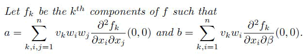
Computation of bifurcation coefficients to determine the local dynamics of the transformed system (14), the value of an and b are computed to probe whether the model system (14) shows forward or backward bifurcation. Since v1=v2=v5=v6=v7=0 for k=1; 2; 5; 6; 7 then k=3; 4; 8; 9 are considered. For the system (14), the associated non-zero second order partial derivatives at disease-free equilibrium and at ε2= ε∗2 are given by
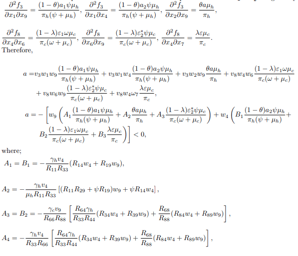

For the value of b, it can be shown that there exists a nonvanishing partial derivative.
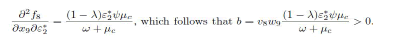
Therefore, a<0 and b>0, hence the model system (1) exhibit a forward bifurcation.
Lemma 6. The unique endemic equilibrium is guaranteed and by 3.2, the model is locally asymptotically stable for R0>1. In addition, by 3.2 item (i), the model undergoes backward bifurcation when a>0. This holds only if v3<0 and v8<0, otherwise it undergoes forward bifurcation.
Results and Discussion
Bifurcation Diagram
Figure 2 illustrates the forward bifurcation (transcritical bifurcation) at R0=1 when a<0 and b>0 for a model system described by equation (1). Thus, the bifurcation diagram for the model system shows that the disease-free equilibrium and endemic equilibria exchange stability when R0=1. This scenario indicates biologically that the model system (1) is globally asymptotically stable at the disease-free level. The equilibrium point emerges when R0<1, and a unique endemic equilibrium point results whenever R0>1. The unique endemic equilibrium point is locally asymptotically stable when R0 is near one. Observably, as R0 decreases below one (R0<1), no endemicity exists, and the disease wanes. As R0 rises above one (R0>1), the disease spreads through the population.

Figure 2: Forward bifurcation diagram for the model system (1) illustrating how that the disease-free equilibrium and endemic equilibria exchange stability when R0=1. The cyan and blue curve indicate stable equilibria whereas the dashed red curve signifies unstable equilibrium.
Global Stability of Endemic Equilibrium Point
This subsection deploys the Lyapunov function method to study the global stability of the Endemic Equilibrium Point (EEP) beyond just the issue of neighborhood equilibrium points. The Lyapunov 25 function enables the extension of the analysis to capture an enormous region, as opposed to relying only on a strip region.
Theorem 3.3. If Re>1, then the bovine tuberculosis disease model system (1) has a unique equilibrium point E∗ which is globally asymptotically stable.
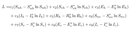
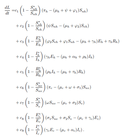
Proof. Since a suitable Lyapunov function is developed using approach, the Lyapunov function will then be applied to analyze the global stability of the endemic equilibrium point of the model system (1). Therefore, the Lyapunov function is developed using the general form as illustrated below:
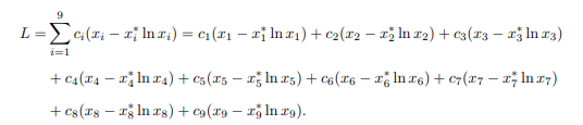
where ci is a positive constant, xi is the population of the ith compartment and x∗i is the endemic equilibrium point. Thus, the following Lyapunov function is constructed:
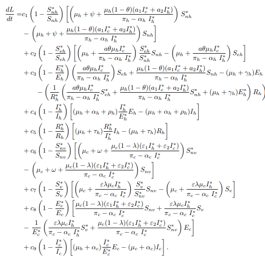
Since the chosen function L and its constant are always differentiable and continuous, the differentiating L regarding time yields the following results:
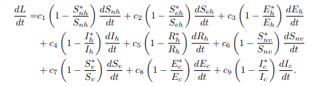
Substituting the model equations of the model system (1) into the equation (18) to obtain
Now, at the endemic equilibrium point of the model system (1) the following are results.
Case 1: Considering the differential equations of human population, then making πh, ψ, τh, γh and ρh the subject yields the following:
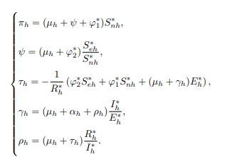
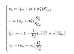
Case 2: Considering the differential equations of cattle population and making πc, ω, (μc+γc) and γc the subject yields the following:
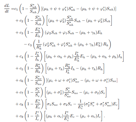
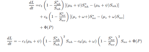
Now, substituting equations (20) and (21) into the equation, then dL/dt becomes.
To investigate the global stability of the endemic equilibrium using the Lyapunov function approach at the steady state, set dN∗h/dt=0 and dN∗c/dt=0, such that:

Substituting equation (23) and (24) into forces of infections to obtain:
After substituting equation (25) into (26), the equation becomes
Simplifying equation (26), it gives
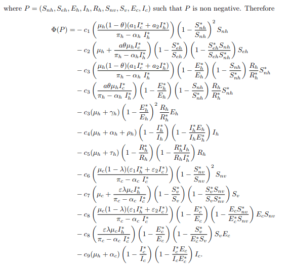
Therefore, following the idea of the function Φ (Snh, Seh, Eh, Ih, Rh, Snv, Sv, Ec, Ic) is non positive, that is Φ (Snh, Seh, Eh, Ih, Rh, Snv, Sv, Ec, Ic) ≤ 0 for all (Snh, Seh, Eh, Ih, Rh, Snv, Sv, Ec, Ic). Then, this implies that dL/dt ≤ 0 for all (Snh, Seh, Eh, Ih, Rh, Snv, Sv, Ec, Ic) and it is zero only when Snh=S∗nh, Seh=S∗eh, Eh=E∗h, Ih=I∗h, Rh=R∗h, Snv=S∗nv, Sv=S∗v, Ec=E∗c, Ic=I∗c. Therefore, the largest compact invariant set in Snh, Seh, Eh, Ih, Rh, Snv, Sv, Ec, Ic such that dL/dt=0 is the singleton (E∗) which is the endemic equilibrium point of the model system (1). [20] principle, indicates that (E∗) is globally asymptotically in the interior region of Snh, Seh, Eh, Ih, Rh, Snv, Sv, Ec, Ic. Now recalling the definition of Lyapunov stability, if L(Snh, Seh, Eh, Ih, Rh, Snv, Sv, Ec, Ic)>0 ∀(Snh, Seh, Eh, Ih, Rh, Snv, Sv, Ec, Ic) ∈ Ω \{E∗}, L(E∗)=0 and L′(Snh, Seh, Eh, Ih, Rh, Snv, Sv, Ec, Ic) ≤ 0 ∀(Snh, Seh, Eh, Ih, Rh, Snv, Sv, Ec, Ic) ∈ Ω \{E∗} then, E∗=(S∗nh, S∗eh, E∗h, I∗ h, R∗ h, S∗nv, S∗v , E∗c , I∗c) is stable. Furthermore, if L(Snh, Seh, Eh, Ih, Rh, Snv, Sv, Ec, Ic)>0 ∀(Snh, Seh, Eh, Ih, Rh, Snv, Sv, Ec, Ic) ∈ Ω\ {E∗}, L(E∗)=0 and L′ (Snh, Seh, Eh, Ih, Rh, Snv, Sv, Ec, Ic)< 0 ∀(Snh, Seh, Eh, Ih, Rh, Snv, Sv, Ec, Ic) ∈ Ω\{E∗} then, E∗=(S∗nh, S∗eh, E∗h, I∗h, R∗h, S∗nv, S∗v, E∗c, I∗c) is asymptotically stable.
Sensitivity and Numerical Analysis
Sensitivity Analysis: The sensitivity analysis helps identify the influence of model parameters on the effective reproduction number (Re) and disease transmission. It determines which parameters and initial conditions affect the model output. Additionally, it informs researchers about which parameters require more numerical attention. The normalized forward sensitivity index of the variable Re depends on the differentiability of a parameter p and is defined as follows:
where ψ is a parameter present in effective reproduction number Re. For example, the sensitivity index of Re corresponding to the parameter α is given as
Other indices are calculated using a similar approach and the results are displayed in Table 2 and Figure 3.
| Parameter |
Sensitivity index |
Parameter |
Sensitivity index |
| a1 |
+3.00524 ×10⁻⁶ |
a2 |
+3.4392 × 10⁻⁸ |
| a |
+1.10214 × 10⁻⁶ |
ε1 |
+1.33268 × 10⁻⁶ |
| ε |
+1.67366 × 10⁻⁶ |
ε2 |
0.999994 |
| ρh |
-2.10205 × 10⁻⁶ |
γh |
+1.32496 × 10⁻⁶ |
| γc |
0.999997 |
µh |
+7.8354 × 10⁻⁷ |
| µc |
0.0694459 |
αh |
-4.34908 × 10⁻⁷ |
| αc |
-0.999997 |
ψ |
-2.61227 × 10⁻⁶ |
| λ |
-0.33333 |
ω |
-0.930551 |
| θ |
-9.11778 × 10⁻⁶ |
- |
- |
Table 2: Sensitivity indices of Re using parameter values in Table 1.

Figure 3: Graph of sensitivity indices of Re with respect to the model parameters.
Interpretation of the Sensitivity
Figure 3 displays the sensitivity profile of Re concerning the model parameters found within Re. Further analysis reveals that the parameters a2, a1, a, ε1, ε2, ε, γh, γc, and μh have positive indices, while μc, ρh, αh, alphac, ψ, λ, ω, and θ have negative indices. Notably, parameters γc and ε2 exhibit index values of +0.999997 and +0.999994, respectively, indicating that an increase in these parameters, while keeping other variables constant, elevates the effective reproduction number Re.
In other words, increasing these parameters heightens the risk of a bTB outbreak in the wider population. To minimize infections in the cattle population, the rates γc and ε2 must be kept sufficiently low to ensure that the removal rate from the exposed to infectious class remains minimal, while also maintaining a low contact rate in contaminated environments and inter-cattle transmission.
On the contrary, the vaccine parameter ω and the induced death rate αc emerge as the most negatively sensitive parameters, with index values of αc=−0.999997 and ω= −0.930551, respectively. This implies that increasing the value of ω by vaccinating healthy cattle and the value of αc by culling infected animals, while keeping other parameters constant, reduces the effective reproduction number Re, thus alleviating the disease burden among the cattle population and promoting disease free conditions in the human population.
Numerical Simulation
The most effective approach for accurately solving an Ordinary Differential Equation (ODE) is to carefully develop an exact solution, as discussed in. The chosen method must always uphold the standard properties of the approximated solution, including consistency and convergence, and it must also preserve the qualitative properties of the solution, such as boundedness and positivity, as highlighted. In this section, we employed the Runge-Kutta fourth (RK4) order method to obtain mathematical results for the model system due to its heuristic properties within the ODE framework. This method is known for its stability and practicality, even with large time steps, as demonstrated in previous studies. We utilized the ODE45 version in MATLAB software to execute the computations using the parameter values presented in Table 1. The initial conditions for the state variables were set as follows: Snh=15000, Seh=1000, Eh=1000, Ih=500, Rh=300, Snv=15000, Sv=10, Ec=6000, and Ic=10. These initial conditions were arbitrarily chosen to illustrate specific behaviors of the model system (Figure 4).
Evolution of Population against Time

Figure 4: Dynamics of human and cattle populations over time with interventions.
Figure 4 depicts the behavior of the infected human and cattle populations as time progresses. Figures 4(a) and 4(b) indicate that interventions for both the human and cattle populations reduce the number of infected individuals significantly. This result attests to the existence of the DFE point in the model system (1). When ψ=0, ρh=0, and ω=0, it implies that interventions are not in place, meaning the populations of humans and cattle can never reach zero, no matter how long the EE point of the model system persists.
Simulation on the effects of varying some parameter values on the model this section presents data derived from the performance of the simulation of model system to explore the behavior of certain state variables over time. This simulation involved varying selected parameter values, as presented in Table 1. The simulation results are graphically displayed in Figure 5.

Figure 5: (a) Effect of education efficacy (θ) on infected human population and (b) Effect of vaccination efficacy (λ) on infected cattle population.
Figure 5 shows that education efficacy (θ) and vaccine efficacy (λ) play pivotal roles in reducing infectious hosts in humans and cattle. Thus, as education and vaccine efficacy approach 1, the number of infectious humans and cattle decreases.
From Figure 6, it can be surmised that the application of rifampicin, isoniazid, ethambutol, and pyrazinamide as medication for infected humans at the rate ρh and Bacille Calmette Gu´erin (BCG) vaccination for infected cattle at the rate ω leads to a reduction in the number of infected humans and cattle when employed on a large scale and applied effectively.

Figure 6: (a) Effect of treatment (ρh) on recovered human population and (b) Effect vaccine (ω) on cattle population.
Figure 6(b) reveals that when cattle are vaccinated to at least ω ≥ 0.4 with a minimum dose of 20 mg, the number of healthy cattle increases rapidly. Additionally, the number of recovered humans also rises, as shown in Figure 6(a). Similarly, when treatment implementation reaches at least ρh ≥ 0.4, it triggers a significant increase in the number of recovered humans.
Simulation on Environmental Contamination
This section presents results from the simulation of the infected human and cattle populations when pastures, soil, slurry, and hay are presumably heavily contaminated with M. bovis, with potential infections stemming from sputum, pus, urine, feces, and other excretions of infectious animals (Figure 7).

Figure 7: Impacts of contaminated environment (ϵ2) on (a) Infected human population and (b) Infected cattle population.
Figure 7(b) illustrates that the number of infected cattle rises as the grazing rate (ϵ2) on the heavily contaminated environment increases. However, after several months, the number of infected cattle decreases due to the disease.
Simulation on Multiple Intervention Strategies
This section presents data derived from simulating the infected human and cattle populations. It explores the outcomes resulting from the execution of various intervention strategies simultaneous (Figure 8).

Figure 8: (a) Impacts of multiple interventions on infected human population and (b) Single intervention on infected cattle population.
Figure 8 shows the effects of a different combination of interventions (public health education campaigns, treatment, and vaccination) on the bTB transmission dynamics. Figure 8 shows that combining all three intervention strategies decreases disease transmission in the endemic area faster than using only two interventions.
Conclusion
This study has presented the formulation of the model for bTB disease transmission in the presence of control strategies, which include public health education campaigns, treatment, and vaccination. Specifically, it has clearly demonstrated the positivity and boundedness of the model system (1) for the model’s domain to be biologically and mathematically meaningful. The results stemming from the sensitivity analysis on all model parameters, aimed at determining their relationship with the effective reproduction number (Re), show that the probability of cattle contracting M. bovis from the contaminated environment, inter-cattle transmission (ε2), and the removal rate from the exposed class to the infectious class (γc) are the most positively sensitive parameters for the effective reproduction number. In contrast, the most negatively sensitive parameters are ω (vaccination) and αc (induced disease death rate), indicating that all infectious cattle are subject to culling in the absence of curative medication administration. Moreover, the numerical simulation of the model reveals that the combination of all interventions has the most significant impact on the control of bTB disease. Therefore, these control measures should be implemented concurrently, especially in endemic areas, to effectively control bTB disease transmission.
Funding Statement
There is no any fund which has been given to support this study.
Declaration of Competing Interest
Authors declare that they have no conflict of interest.
Credit Authorship Contribution Statement
Sylas Oswald: Conceptualization, methodology, software, formal analysis, visualization, investigation and writing original draft
Theresia Crispin Marijan and Goodluck Mika Mlay: Conceptualization, methodology, formal analysis, investigation, writing, review, editing, resources and supervision.
Winifrida Benedict Kidima: Biology aspect visualization, investigation, writing, review, editing and supervision.
Acknowledgment
We acknowledge and thank the College of Natural and Applied Science (CoNAS) for the regular moral supports given to the all authors during writing this paper.
References
- Aldila D, Latifah SL, Dumbela PA (2019) Dynamical analysis of mathematical model for Bovine Tuberculosis among human and cattle population. Commun Biomath Sci. 2(1): 55-64.
[Crossref] [Google Scholar]
- Al-Obeidi AS, Al-Azzawi SF (2022) A novel six-dimensional hyperchaotic system with selfexcited attractors and its chaos synchronisation. Int J Comput Sci Math. 15(1):72-84.
[Crossref] [Google Scholar]
- Ashgi R, Pratama MAA, Purwani S (2021) Comparison of Numerical Simulation of Epidemiological Model between Euler Method with 4th Order Runge Kutta Method. Int J Oper Res. 2(1):37-44.
[Crossref] [Google Scholar]
- Ayele WY, Neill SD, Zinsstag J, Weiss MG, Pavlik I (2004) Bovine tuberculosis: an old disease but a new threat to Africa. Int J Tuberc Lung Dis. 8(8):924-937.
[Google Scholar] [PubMed]
- Butcher JC (1996) A history of Runge-Kutta methods. Appl Numer Math. 20(3):247-260. [Crossref]
[Google Scholar]
- Castillo-Chavez C, Song B (2004) Dynamical models of tuberculosis and their applications. Math Biosci Eng. 1(2):361.
[Google Scholar] [PubMed]
- Mdegela RH, Kusiluka LJM, Kapaga AM, Karimuribo ED, Turuka FM, et al. (2004) Prevalence and determinants of mastitis and milk borne zoonoses in smallholder dairy farming sector in Kibaha and Morogoro districts in Eastern Tanzania. J Vet Med B. 51(3):123-128.
- Chitnis N, Hyman JM, Cushing JM (2008) Determining Important Parameters in the Spread of Malaria through the Sensitivity Analysis of a Mathematical Model. Bull Math Biol. 70(5):1272.
[Crossref] [Google Scholar] [PubMed]
- Diekmann O, Heesterbeek JAP, Metz JA (1990) On the definition and the computation of the basic reproduction ratio R0 in models for infectious diseases in heterogeneous populations. J Math Biol. 28(4):365-382.
[Crossref] [Google Scholar] [PubMed]
- Dumont Y, Chiroleu F, Domerg C (2008) On a temporal model for the Chikungunya disease: modelling, theory and numerics. Math Biosci. 213(1):80-91.
[Crossref] [Google Scholar] [PubMed]
- Durnez L, Sadiki H, Katakweba A, Machang’u RR, Kazwala RR, et al. (2009) The prevalence of Mycobacterium bovis-infection and a typical mycobacterioses in cattle in and around Morogoro, Tanzania. Trop Anim Health Prod. 41(8):1653-1659.
[Crossref] [Google Scholar] [PubMed]
- Ekwem D, Morrison TA, Reeve R, Enright J, Buza J, et al. (2021) Livestock Movement Informs the Risk of Disease Spread in Traditional Production Systems in East Africa. Sci Rep.
[Crossref] [Google Scholar] [PubMed]
- Hassan AS, Garba SM, Gumel AB, Lubuma JS (2014) Dynamics of Mycobacterium and bovine tuberculosis in a human-buffalo population. Comput Math Method Med.
[Crossref] [Google Scholar]
- Hyera EM, Athumani SN (2017) The status and characteristics of two populations of small East African goats of Tanzania.
[Google Scholar]
- Kamgang JC, Sallet G (2005) Global asymptotic stability for the disease free equilibrium for epidemiological models. C R Math. 341(7):433-438.
[Crossref] [Google Scholar]
- Karimuribo ED, Ngowi HA, Swai ES, Kambarage DM (2007) Prevalence of brucellosis in crossbred and indigenous cattle in Tanzania. 19(10):148-152.
[Google Scholar]
- Katale BZ, Mbugi EV, Matee MI, Fyumagwa RD, Keyyu JD, et al. (2012) Bovine tuberculosis at the human-livestock-wildlife interface: is it a public health problem in Tanzania? A review: proceedings. 79(2):1-8.
[Google Scholar]
- Korobeinikov A, Wake GC (2002) Lyapunov functions and global stability for SIR, SIRS, and SIS epidemiological models. Appl Math Lett. 15(8):955-960.
[Crossref] [Google Scholar]
- LaSalle JP (1976) The stability of dynamical systems.
[Google Scholar]
- Liu S, Li A, Feng X, Zhang X , Wang K (2016) A dynamic model of human and livestock tuberculosis spread and control in Urumqi, Xinjiang, China. Comput Math Method Med.
[Crossref] [Google Scholar] [PubMed]
Citation: Oswald S, Marijani TC, Mlay GM, Kidima WB (2025) Mathematical Modelling of Bovine Tuberculosis
Transmission Dynamics: Role of Combination of Control Measures. J Veterinary Med. 09:41.
Copyright: © 2025 Oswald S, et al. This is an open-access article distributed under the terms of the Creative Commons
Attribution License, which permits unrestricted use, distribution, and reproduction in any medium, provided the original author
and source are credited.