Research Article - (2025) Volume 33, Issue 2
Comparison Between the KNN, W-KNN, Wc-KNN and Wk-KNN Models on a CDC Heart Disease Dataset
Andre Fix Ventura*
Department of Pharmaceutics, Universidade do Estado da Bahia, Salvador, Brazil
*Correspondence:
Andre Fix Ventura, Department of Pharmaceutics, Universidade do Estado da Bahia, Salvador,
Brazil,
Email:
Received: 03-Jun-2024, Manuscript No. IPQPC-24-20344;
Editor assigned: 05-Jun-2024, Pre QC No. IPQPC-24-20344 (PQ);
Reviewed: 19-Jun-2024, QC No. IPQPC-24-20344;
Revised: 20-Mar-2025, Manuscript No. IPQPC-24-20344 (R);
Published:
27-Mar-2025, DOI: 10.36648/1479-1064.33.2.52
Abstract
One of the most popular and fundamental methods used for machine learning classification is KNN (KNearest Neighbor). Despite its simplicity, this method can achieve good data classification results even without prior knowledge of the data distribution. WKNN (Weighted KNN) is an improvement of KNN in which, instead of merely counting the number of nearby neighbors, the system assigns a weight to each neighbor. Typically, this weight is defined by the inverse of the squared distance (weight=1/d2). This study aims to present an alternative way to define the weight (weight=wp/(1+|cd|n) and a methodology in which the weight formula is defined based on the position and the training data. It was found that, in this dataset, the presented methodology achieves results that are 9% better than KNN and 8% better than WKNN.
Keywords
Drug-drug interactions; Knowledge; Medication; Pharmacy professionals
Introduction
One of the challenges of machine learning is to accurately classify a given piece of data into a list of classification possibilities. The data are described by a set of attributes (or features). Its classification can be:
Binary classification: A yes/no response, such as whether a patient has a certain disease or not.
Multiclass classification: This can be one possibility from a pre-known list of possibilities, for example, determining the specie to which an animal belongs.
One vs. Rest classification (OvR): This method simplifies multiclass classification into several binary problems in which a specific class is trained against all other options.
One vs. One classification (OvO): This method simplifies multiclass classification into several binary problems in which two specific classes are compared against each other.
Multilabel classification: Determine which characteristics are present or not present in a sample. For example, tagging a text indicates its characteristics, such as emotional, formal, political, or economic characteristics.
Others: There are other classifications, such as hierarchical and probabilistic, but they are not the focus of this study.
Just as there are various types of classification, there are several methodologies for a machine learning classifier, such as the following:
Logistic regression: This model is used in binary classifications where a logistic (sigmoid) function models the probability of an observation belonging to a certain class. Despite being simple, interpretable, and performing well, it is less effective for nonlinear problems [1].
Decision tree: The data are split into subgroups based on their characteristics, thus creating a data tree. While interpretable and capable of capturing nonlinear relationships, it is prone to overfitting and sensitive to small variations in the data [2].
Random forest: A collection of multiple decision trees trained on different subsets of data. Although this approach reduces the overfitting effect of a single decision tree, it is less interpretable than an individual tree [3].
Support Vector Machines (SVM): Finds the hyperplane that best separates the classes in the feature space. While effective in high-dimensional spaces, it is essentially linear. To address linearity, the kernel trick can be used, but choosing the right kernel can be challenging [4].
k-Nearest Neighbors (k-NN): Classifies the observation based on the classes of data points close to the analyzed sample. Despite being simple to implement and not making assumptions about the data distribution, this approach can be slow for large datasets, sensitive to outliers and the choice of k value is crucial.
Naive Bayes: Classification is based on Bayes' theorem. While fast, effective in problems with many features, and robust when applied to small datasets, it is assumed that features are independent, which is rarely true. When features are highly related, the algorithm may perform poorly [5].
Artificial Neural Networks (ANN): Learn complex patterns through adjustable weights in multiple layers of neurons. While capable of modeling complex and nonlinear relationships, this approach requires large amounts of data and computational power. Additionally, it is difficult to interpret [6].
Gradient Boosting Machines (GBMs): These above models are combined, and each model corrects the errors of the previous models. While having excellent performance and the ability to handle nonlinear data, it can be slow to train and run, prone to overfitting if not well regulated, sensitive to parameters, and less interpretable. Extreme gradient boosting (XGBoost), LightGBM, and CatBoost are some variants of GBM [7].
In this vast spectrum of methodologies, this study focuses on k-NN, which is a nonlinear system that makes no assumptions about the data distribution. Although slow for large datasets, this model typically provides more accurate responses than do the other mentioned methodologies.
One of the main disadvantages of this model is its sensitivity to outliers, meaning that the presence of atypical points (incorrect or poorly collected) can significantly affect the prediction.
This study aims to minimize the impact of outliers and thereby achieve a more accurate response.
Materials and Methods
Dataset
The dataset used in this research is called Indicators of Heart Disease The study indicated that “According to the CDC, heart disease is a leading cause of death for people of most races in the U.S. (African Americans, American Indians and Alaska Natives, and whites). About half of all Americans (47%) have at least 1 of 3 major risk factors for heart disease: High blood pressure, high cholesterol, and smoking. Other key indicators include diabetes status, obesity (high BMI), not getting enough physical activity, or drinking too much alcohol. Identifying and preventing the factors that have the greatest impact on heart disease is very important in healthcare. In turn, developments in computing allow the application of machine learning methods to detect "patterns" in the data that can predict a patient's condition.
The dataset originally comes from the CDC and is a major part of the Behavioral Risk Factor Surveillance System (BRFSS), which conducts annual telephone surveys to collect data on the health status of U.S. residents. As described by the CDC: "Established in 1984 with 15 states, BRFSS now collects data in all 50 states, the District of Columbia, and three U.S. territories. BRFSS completes more than 400,000 adult interviews each year, making it the largest continuously conducted health survey system in the world. The most recent dataset includes data from 2023. In this dataset, I noticed many factors (questions) that directly or indirectly influence heart disease, so I decided to select the most relevant variables from it.”
In this study, we utilized a subset containing only 50,000 samples, despite the dataset having more than 400,000 samples.
We performed an initial data treatment to ensure that all the values were normalized between 0 and 1. To achieve this, we identified the minimum and maximum values for each feature and applied the following formula’
normalized value=(value-min)/ (max-min)
The values "Yes" and "No" were considered "Yes" with a value of 1 and "No" with a value of 0 [8,9].
Performance evaluation
To evaluate the performance of the system, we utilized a widely used standard for measuring the effectiveness of a model. First, we categorized the system's responses into four types.
TP or True Positive: The system returns positive, and the sample also indicates positive.
TN or True Negative: The system returns negative, and the sample also indicates negative.
FP or False Positive: The system returns positive, but the sample indicates that it should be negative.
FN or False Negative: The system returns negative, but the sample indicates that it should be positive (Table 1).
| Measure |
Formula |
| Accuracy |
TP+TN/TP+TN+FP+FN |
| Error rate |
FP+FN/TP+TN+FP+FN |
| Specificity |
TN/TN+FP |
| Precision |
TP/TP+FP |
| Recall |
TP/TP+FN |
| F1 Score |
2(Presion*recall)/presion+ recall |
Table1: Performance evaluation.
Cross Validation
To improve the model evaluation described in section 2.2, the technique of cross-validation with shuffling was used.
This technique involves shuffling all samples and then dividing the dataset of 50,000 samples into 10 groups of 5,000 samples each. Nine of these groups are used to train the model, and the 10th group is used to test the model.
This procedure was repeated 10 times, and the final result was the average of the 10 obtained samples.
This approach eliminates the bias influenced by the order of the samples and reduces statistical randomness, as each presented result is an average of the outcomes.
KNN Algorithm
The K-Nearest Neighbor (KNN) algorithm aims to determine the classification (or simply, class) of a sample based on a training dataset. Each sample in the dataset and the input sample are a set of fields (or features), which are typically numerical, boolean, or a list of possibilities. These fields are also referred to as features.
For this document, we will refer to a sample as a set of features. If it is a training sample, the result of the sample's features, i.e., the class in which the sample is classified, will also be part of the sample.
The methodology involves having a set of samples, called a dataset, as input for training, specifying a number k of nearby samples, and the input data.
The system then searches for the k nearest elements in the provided dataset using one of the distance calculation formulas described.
Among these k elements, how many elements belong to each class is checked. The class with the most elements is indicated as the response.
WKNN Algorithm
The objective of weighted KNN (WKNN) is the same as that of KNN, but its calculation is slightly different. In this case, there is no fixed number of k elements but rather a weight for each sample.
The weight calculation is typically given by w=1/d2, although there are studies with other formulas [10-15]. In this calculation, d is the distance between the input and each of the samples.
If the sample is of this class, the weights for each class are summed. The class with the highest total weight is the class indicated as the response.
The suggested weight formula
In this section, we analyze an alternative suggestion for the weight calculation formula. The total weight (wt), defined as wt=1/d2 poses some challenges because when the distance approaches zero, the weight tends to infinity, as shown in the figure below. When we analyze some locations that are very close to a certain neighbor, the other neighbors are completely ignored, possibly leading to false positives if the neighbors have some outliers some challenges because when the distance approaches zero, the weight tends to infinity, as shown in the figure below. When we analyze some locations that are very close to a certain neighbor, the other neighbors are completely ignored, possibly leading to false positives if the neighbors have some outliers (Figure 1).

Figure 1: Weight calculation formula.
On the other hand, the formula wt=1/(1+d2) results in a maximum function value of 1 and a minimum value of 0; thus, no neighbor, even a very close neighbor, is overly weighted (Figure 2).

Figure 2: Weight calculation graph.
If we evolve the formula to wt=1/(1+(cd)2). We can calculate a crucial value for this study, which is c when w=50%.
wt= 1/(1+(cd)2)=50%=0.5
0.5 × (1+(cd)2)=0.5+0.5(cd)2=1
0.5(cd)2=0.5
C2=1/d2
c=1/d
Thus, the inverse of c indicates the distance at which the weight is 50%. Therefore, we name this variable “closeness,” or simply c.
Evolving the formula to wt=1/(1+|cd|n, we can see that n indicates the distribution. In the figure below, red represents n=1, blue represents n=2, green represents n=5, purple represents n=10 and black represents n=100 (Figure 3).

Figure 3: WKNN algorithm.
The variable “probability” (p) is added (wt=wpp/1+|cd|n and indicates the probability that the classification at distance d is the selected classification. This probability is calculated by counting the items of the selected classification at this position (qcs) and dividing by the sum of the items with the selected classification and the items with other classifications (qcns), i.e.,
p=qcs/(qcs+qcns)
Finally, the weight at position (wp) indicates the weight to be considered at that position. In this study, the weight of each data point is always the same regardless of which classification it is related to; thus, the weight is simply the sum of items at that specific position.
For example, if we have 3 points at a certain position, with 2 belonging to class A and 1 to class B, considering n=2 and c=1, the wt for class (Figure 4).
A would be
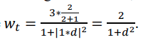

Figure 4: WKNN algorithm.
If we have n=1000 and c is equal to the inverse of the distance of the 3rd nearest element, the weights of the 2 nearest elements would tend to 100%, and the weight of the 3rd element would be 50%.
Under these conditions, the system closely resembles traditional KNN for k=3 elements, with the only difference being that the third element will have a weight of 50% instead of 100%.
Similarly, if c is a large value, if wp=c2 and n=2, the equation tends to w=wp/(1+(cd)2) ≅ c2/c2d2, which is close to WKNN with a weight equal to the inverse of the square distance. In the figure below, we have w=1002/(1+(100d)2) (Figure 5).

Figure 5: WKNN algorithm.
Thus, the proposed formula can approximate both the KNN and WKNN results depending on the selected parameters. This unified formula allows further analyses.
Distance x Position
There are several ways to calculate the distance between two points, as shown by: [10]
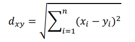
Euclidean distance
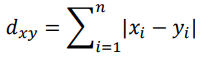
Manhattan distance
Minkowski distance
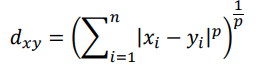
Note that if p=1, it is equal to the Manhattan distance, and if p=2, it is equal to the Euclidean distance.
Chebyshev distance
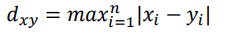
The greatest value of the individual distance in each dimension.
Weighted distance
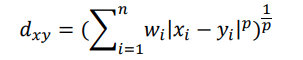
It is a variation of the Minkowski distance, where wi is the weight of the distance in each dimension.
Among these methods, the most complete is the weighted distance method. However, for simplicity, in this study, we use the Euclidean distance. In the above equations, there are various methods for calculating the distance between points X and Y in N dimensions, where X and Y are vectors of N dimensions. Now, let us determine that X is the input vector for which the system calculates the classifications, and Y is the position pi of training sample index i.
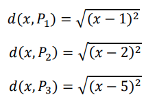
To facilitate understanding, consider the following example: we have a 1-dimensional space with 3 points. Point X=(1) is of class A, point X=(2) is of class B, and point X=(5) is of class A. In this scenario, we can calculate the distances as follows:
Considering wt=wpp/(1+|cd|n), with wpp=1 and n=2, we have the formula w (x, pi)=1/(1+c2 × (x−pi)2). We define the space covered by a certain class as the sum of the weights of each sample P of that class, i.e.,
In this example, considering c=1/0.1, we have the following coverage (Figures 6 and 7).

Figure 6: Plot of two sharp Lorentzian peaks centered at x=1 and x=5.
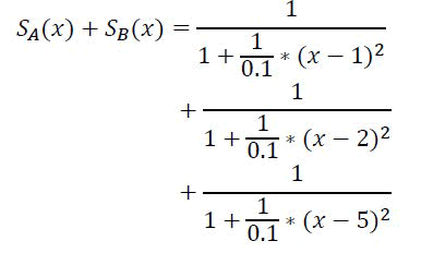

Figure 7: Plot of a periodic function with sharp peaks, resembling a sum of Lorentzian distributions.
According to the graphs above, the peaks occur exactly at the positions of the samples, i.e., at points 1, 2, and 5, and the width of the peaks is approximately 0.1 on each side at 50% of their height (Figure 8).

Figure 8: Graph of a sharp peak function showing rapid growth and decay near x=1.
Thus, as seen both theoretically and in the example above, the formulas consider not the concept of distance between points but the concept of a space formula S for the selected class, considering the positions of each sample and, as input, the vector X.
WKNN Algorithm with the Proposed Weight Formula
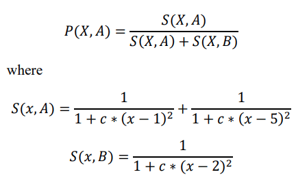
As previously shown, for each class, there is a space defined by the training samples as follows.
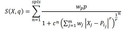
where X is the vector of the position to be calculated. q is the class to be calculated. wp is the weight of class q at position P. wj is the weight of dimension j. p is the probability of this sample being of class q. c is the closeness. n is the distribution of the data. m is the number of dimensions of vector X and vector P.
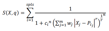
r is the factor of the distance calculation according to the Minkowski distance. pi is the vector that defines the position of sample i. Spls is the number of samples. In this study, we define wp=1, r=2, wj=1; thus, this formula simplifies to:
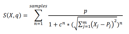
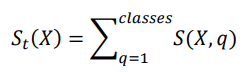
The total space is defined as the sum of the spaces of each class.
The probability of position X being of class q is defined as
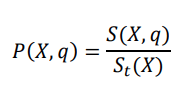
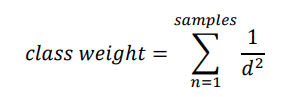
The coverage rate is determined by analyzing whether sufficient data exist in the calculated region. These data are important because if there is low coverage, the calculation may be unreliable. Thus, the coverage rate of the calculation is defined as.
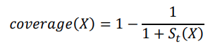
For clarity, let us return to the previously cited example of 3 points where we have the point X=(1) belonging to class A, the point X=(2) belonging to class B, and the point X=(5) belonging to class A. We can calculate the probability of position X being of class A as follows:
The graph below represents the probability of position X being classified as class A based on the 3 training points. The black line in the graph represents c=1/0.1, the red line represents c=1/0.2 and the blue line represents c=1/0.4. The second graph indicates the probability of being classified as class B, and the third graph shows the coverage rate of the calculation for the same values of c (Figure 9).

Figure 9: Visualization of different kernel functions and their effects.
Combining the first two graphs for c=1/0.4, we have the green line representing class A and the blue line representing class B. The system will classify as B in the region where X is between 1.507 and 3.33, and in the other regions, the system will classify as A (Figure 10).

Figure 10: Interference of two sine waves creating a beat pattern.
In addition to just classifying, the system outputs the probability of the generated classification and the coverage rate. For example, in the graph above, the value x=2 has an 86.6% chance of being class B, with a coverage rate of 98.1%. Moreover, the value x=3 is also classified as class B, but with a probability of 64.8% and a coverage rate of 15.3%. This occurs because the position x=3 is further from the samples.
Wc-KNN and Wk-KNN
We named the calculation of the final probability Wc-KNN, as described previously, considering “c” as an input to the system and, therefore, a constant.
The Wk-KNN works slightly differently. This methodology considers the formula described but also takes k into account in a manner similar to traditional KNN.
Thus, the system first checks the k-th nearest sample and uses the formula c=1/d, where d is the distance to the k-th sample.
With this, we ensure that the k-th element has S(X)=0.5 and that the remaining items closer than the k-th element have S(X) ≥ 0.5. Consequently, we can state that St(X) ≥ k/2, which ensures that the calculation will be performed with a significant number of samples with S(X) ≥ 0.5.
Multiclass e Multilabel
As previously discussed, we can calculate the probability of a given position X being classified into each of the trained classes.
Since each class is calculated independently, this study will be limited to calculating only the probability of a given position being in a specific class. In this case, we will analyze only the class "heart disease" (and consequently, "no heart disease").
In multiclass systems, the classes are mutually exclusive; thus, the class with the highest probability is the class in which position X is classified.
The multilabel classification operates differently. In both the training and the results, a given position can be classified with zero, one, or more classes. For example, a patient's clinical examination may indicate that he is healthy or has one or more diseases according to a list of tested diseases.
In this case, the system should calculate as described earlier, but the result should be analyzed with a percentage threshold instead of just verifying what is most probable. Additionally, the training data may indicate that a given position has more than one classification.
To determine the percentage threshold value, we verify the average percentage of the sample in the training data. If the percentage offered by the system is higher than the average percentage of the sample, the result is considered positive, meaning that the point is classified as belonging to the analyzed class. A lower value is considered negative, meaning that the point does not belong to the class.
Comparison between the Models
The main idea is to implement the four models described, prepare the dataset, calculate the formulas according to the cross validation method, and compare the performance of each model by evaluating the results obtained from the formulas outlined.
Results
The results obtained by running the four models on the dataset from section 2.1 are presented in this section (Tables 2-5).
| K |
Accuracy (%) |
Error rate (%) |
Specificity (%) |
Precision (%) |
Recall (%) |
F1 score (%) |
| 3 |
80.06 |
19.94 |
83.59 |
16.2 |
39.58 |
22.99 |
| 5 |
74.67 |
25.33 |
74.81 |
27.21 |
73.48 |
39.71 |
| 10 |
66.67 |
33.33 |
64.55 |
16.87 |
95.24 |
28.67 |
| 100 |
75.5 |
24.5 |
75.25 |
23.89 |
77.21 |
36.49 |
Table 2: The KNN model achieved the following results.
| Accuracy (%) |
Error rate (%) |
Specificity (%) |
Precision (%) |
Recall (%) |
F1 score (%) |
| 81.2 |
18.8 |
83.92 |
23.36 |
49.25 |
31.69 |
Table 3: The WKNN model achieved the following results.
| N |
C |
Accuracy (%) |
Error rate (%) |
Specificity (%) |
Precision (%) |
Recall (%) |
F1 score (%) |
| 2 |
0.01 |
76 |
24 |
79.87 |
23.95 |
46.67 |
31.66 |
| 1 |
0.01 |
81.33 |
18.67 |
84.96 |
23.67 |
41.52 |
30.15 |
| 1 |
0.005 |
82.8 |
17.2 |
85.47 |
29.58 |
55.22 |
38.53 |
| 1 |
0.004 |
83.67 |
16.33 |
85.06 |
36.25 |
71.52 |
48.11 |
| 1 |
0.002 |
86 |
14 |
87.5 |
29.29 |
66.67 |
40.69 |
| 1 |
0.0015 |
85.67 |
14.33 |
88.83 |
27 |
47.62 |
34.46 |
| 1 |
0.001 |
86.67 |
13.33 |
87.76 |
29.68 |
70.64 |
41.8 |
| 1 |
0.0001 |
85 |
15 |
87.95 |
16.85 |
37.5 |
23.25 |
| 1.5 |
0.0015 |
81 |
19 |
83.17 |
22.75 |
56.29 |
32.4 |
| 0.5 |
0.0015 |
85.4 |
14.6 |
88.95 |
26.01 |
42.17 |
32.17 |
Table 4: The Wc-KNN model was tested with various configurations, varying N and C. The best results for this dataset were for C=0.002 and N=1, with an accuracy of 86%.
| N |
K |
Accuracy (%) |
Error rate (%) |
Specificity (%) |
Precision (%) |
Recall (%) |
F1 score (%) |
| 2 |
5 |
83.3 |
16.7 |
85.84 |
26.64 |
57.88 |
36.48 |
| 2 |
10 |
79.33 |
20.67 |
80.1 |
18.48 |
61.31 |
28.4 |
| 2 |
100 |
83.67 |
16.33 |
85.36 |
30.91 |
70.94 |
43.06 |
| 2 |
250 |
84.33 |
15.67 |
88.85 |
31.44 |
44.85 |
36.97 |
| 1 |
3 |
80.67 |
19.33 |
83.12 |
19.12 |
48.98 |
27.51 |
| 1 |
5 |
81.67 |
18.33 |
86.05 |
20.87 |
37.62 |
26.85 |
| 1 |
10 |
84.33 |
15.67 |
87.7 |
27.61 |
49.97 |
35.57 |
| 1 |
11 |
85.67 |
14.33 |
88.18 |
22.73 |
54.04 |
32 |
| 1 |
12 |
86.67 |
13.33 |
88.88 |
29.68 |
62.5 |
40.25 |
| 1 |
13 |
85.33 |
14.67 |
87.99 |
27.62 |
53.71 |
36.48 |
| 1 |
32 |
86 |
14 |
88.28 |
23.75 |
49.52 |
32.1 |
| 1 |
100 |
87.33 |
12.67 |
93.28 |
38.53 |
35.73 |
37.08 |
| 1 |
250 |
86.33 |
13.67 |
89.37 |
35.08 |
55.07 |
42.86 |
| 1 |
500 |
85.33 |
14.67 |
90.96 |
35.35 |
40.55 |
37.77 |
| 1.5 |
10 |
83.33 |
16.67 |
85.01 |
30.49 |
67.51 |
42 |
| 1.5 |
100 |
84 |
16 |
87.43 |
25.93 |
43.85 |
32.58 |
| 1.25 |
100 |
84.67 |
15.33 |
86.28 |
31.93 |
67.22 |
43.29 |
| 1.125 |
100 |
85.67 |
14.33 |
88.74 |
31.09 |
50.17 |
38.39 |
| 0.75 |
100 |
86.1 |
13.9 |
90.01 |
31.18 |
45.96 |
37.15 |
| 0.5 |
100 |
87.1 |
12.9 |
91.55 |
24.39 |
33.18 |
28.11 |
Table 5: The Wk-KNN model was also tested with various configurations, and the best result was obtained for N=1 and K=100,for which the accuracy was 87.33%.
After the data were collected, an evaluation of the obtained data was performed (Table 6).
| Model |
Accuracy (%) |
Error rate (%) |
Specificity (%) |
Precision (%) |
Recall (%) |
F1 score (%) |
| KNN |
80.06 |
19.94 |
83.59 |
16.2 |
39.58 |
22.99 |
| WKNN |
81.2 |
18.8 |
83.92 |
23.36 |
49.25 |
31.69 |
| Wc-KNN |
86 |
14 |
87.5 |
29.29 |
66.67 |
40.69 |
| Wk-KNN |
87.33 |
12.67 |
93.28 |
38.53 |
35.73 |
37.08 |
Table 6: In summary, the table below presents the best results from each of the four models.
It was observed that none of the four models achieved a high F1 score, suggesting that the features used in the dataset are not sufficient to accurately predict whether a patient will have heart disease.
Despite this, the system achieved an accuracy of more than 87% and a precision of more than 38%, which means that if the system generates a positive signal, it is recommended that the patient check their health condition, as more than 1 in 3 positives will indeed indicate heart disease (Table 7).
| Model |
Accuracy (%) |
Error rate(%) |
Specificity (%) |
Precision (%) |
Recall (%) |
F1 score (%) |
| KNN |
100% |
100% |
100% |
100% |
100% |
100% |
| WKNN |
101% |
94% |
100% |
144% |
124% |
138% |
| Wc-KNN |
107% |
70% |
105% |
181% |
168% |
177% |
| Wk-KNN |
109% |
64% |
112% |
238% |
90% |
161% |
Table 7: Good calibration of the models, the Wk-KNN model is likely to achieve better performance. Considering the performance of the KNN algorithm as a baseline, the performance on this dataset was as follows.
These data suggest that adopting the Wk-KNN model can lead to, depending on the dataset, a 9% better accuracy, 138% better precision, and 61% better F1 score than can the KNN model.
Discussion
Using a methodology that considers the weight of the sample based on the distance has proven effective, and the formula used to define both the distance and the weight based on the distance can significantly alter the final result.
This study was limited to comparing the four methodologies and revealed that further exploration of the Wc-KNN and Wk- KNN methodologies could yield more precise results.
As a suggestion for both cases, I recommend a study considering the calculation of "Weighted distance," defining the weight through an iterative process, such as Gradient Descent. For the Wc-KNN model, it is also possible to individualize the 'c' for each sample.
Conclusion
Thus, a suggested study is an iterative system that defines the values of wj, ci, r and n. A suggestion for a start value for wj could be the correlation between the feature values and the sample results.
References
- Brightwood S (2024) Regularization Techniques in Logistic Regression.
[Google Scholar]
- Meng L, Bai B, Zhang W, Liu L, Zhang C (2023) Research on a Decision Tree Classification Algorithm Based on Granular Matrices. Electronics. 12(21):4470.
[Crossref] [Google Scholar]
- Oktafiani R, Hermawan A, Avianto D (2024) Max Depth Impact on Heart Disease Classification: Decision Tree and Random Forest. 8(1):160-168.
[Crossref] [Google Scholar]
- Hoque R, Billah M, Debnath A, Hossain SS, Sharif NB (2024) Heart Disease Prediction using SVM. Int J Sci Res Arch. 11(2):412-20.
[Google Scholar]
- Subarkah P, Damayanti WR, Permana RA (2022) Comparison of correlated algorithm accuracy Naive Bayes Classifier and Naive Bayes Classifier for heart failure classification. 14:120-125.
[Crossref] [Google Scholar]
- Chen Q, Ma N (2024) Heart Disease Prediction Method Based on ANN. Highl Sci Eng Technol. 85:411-417.
[Crossref] [Google Scholar]
- Yu Q, Fu M, Hou Z, Wang Z (2024) Elucidating predictors of preoperative acute heart failure in elderly patients with hip fractures through machine learning and SHAP analysis: a retrospective cohort study.
[Google Scholar]
- Pytlak K (2023) Indicators of heart Disease.
[Google Scholar]
- Hossin M, Sulaiman MN (2015) A review on evaluation metrics for data classification evaluations. Int J Data Model Knowl Manag. 5(2):1.
[Google Scholar]
- Tarakci F, Ozkan IA (2021) Comparison of classification performance of kNN and WKNN algorithms. Selcuk Univ J Eng Sci. 20(2):32-37.
[Google Scholar]
- Fan GF, Guo YH, Zheng JM, Hong WC (2019) Application of the weighted k-nearest neighbor algorithm for short-term load forecasting. Energies. 12(5):916.
[Crossref] [Google Scholar]
- Peng X, Chen R, Yu K, Ye F, Xue W (2020) An improved weighted K-nearest neighbor algorithm for indoor localization. Electronics. 9(12):2117.
[Crossref] [Google Scholar]
- Samad A, Taze S, Uçar MK (2024) Enhancing milk quality detection with machine learning: A comparative analysis of KNN and distance-weighted knn algorithms. Int J Innov Sci Res Technol. 9(3):2021-2029.
[Google Scholar]
- Karabulut B, Arslan G, Ünver HM (2019) A weighted similarity measure for k-nearest neighbors algorithm. 15(4):393-400.
[Google Scholar]
- Pandey S, Sharma V, Agrawal G (2019) Modification of KNN algorithm. 8(11):24869-24877.
[Google Scholar]
Citation: Ventura AF (2025) Comparison between the KNN, W-KNN, Wc-KNN and Wk-KNN Models on a CDC Heart Disease
Dataset. Qual Prim Care. 33:52.
Copyright: © 2025 Ventura AF. This is an open-access article distributed under the terms of the Creative Commons Attribution
License, which permits unrestricted use, distribution, and reproduction in any medium, provided the original author and source
are credited.