Keywords
Gross Domestic Product (GDP), Augmented Dickey-Fuller (ADF) test, Auto
Regressive Distributed Lag (ARDL).
Introduction
Given the complexity of the agriculture workforce, skills and training issues, a strategic and
integrated approach between government and industry is crucial to addressing the issues.
Challenges such as the global financial crisis, food security and climate change have created
some uncertainty about future labor market trends, but the skills and labor demands of the
agriculture industry are expected to grow, particularly given the long term demographic trends.
Training workforce in agricultural sector aims to change behavior at the work place in order to
stimulate efficiency and higher performance standards. It is concerned with work-based learning.
In turn, learning is seen as a form of behavioral change. Training has been usefully defined as
“the systematic development of the attitude, knowledge and skill and behavior pattern required
by an individual in order to perform adequately a given task or job. Participative Management is
one of the most popular and most commonly practiced management styles in modern
organizations. Every organization has leaders who lead the organization to its ultimate objectives
by setting the vision and mission and making sure these are implemented. The roles of leaders
include not just the performance of all these duties and responsibilities but also the need to
connect with their employees and to strike a note in their hearts. This is necessary to help ensure
that the employees are willing to follow their leaders in whatever direction is desired. Human
Resource Development (HRD) professionals also play a crucial role in terms of leadership
management in each organization. Their duties involve not only recruitment, orientation,
provision of training courses, coaching, enforcing organization’s rules and regulations, and
finally removing unwanted employees but, also, core duties, especially in innovative
organizations, focus on strategic planning to create learning organizations and develop
employees to have more potential and competencies.
Building workforce planning and human resource management skills in the industry is necessary
to improve business performance, better equip the industry to respond and adapt to changes, and
increase the industry’s capacity to sustain productivity growth. There is a growing need for
employers in agriculture to develop and implement appropriate workforce planning strategies.
These strategies will help employers establish workplaces that attract and retain staff and which
also better manage issues associated with skills gaps and shortages, the ageing workforce,
evolving service demands and changing market and climate conditions. Nowadays, Human
Resource Management (HRM) is one of the key success factors used for analyzing the internal
environment of organizations, since it acts something like an indicator to measure the
competitive advantages that organizations may have, especially in the newly-emerging world of
the information or knowledge age [1]. The core objective of analyzing human resources in
organization is to consider their weaknesses and the strengths and to compare them with business
competitors. Consequently, HRM is now represented at the highest level of management
[2].Furthermore, it is necessary to consider both HRM and HRD, which involves the deliberate
and planned attempt to improve the quality of human resources with respect to their ability to be
productive at work and to fulfill defined organizational goals. Consequently, both HRM and
HRD professionals are increasingly involved in planning and executing corporate strategies. This
is because, in a world in which supply of many basic products have either become commodities
or for which supply exceeds primarily from the ability of people to create added value in one
way or another. The primary HRD functions are training and development, organizational
development and career development [3]. Nevertheless, HRD professionals also perform
functions similar to public relations staff members who connect owners, board members and
committees, employers and employees [4]. With these distinguishing roles and duties, HRD
professionals currently have to enhance their competencies and use them in the proper directions
and to promote sustainability as well. Generally, therefore, HRD professionals have powerful
tools available to encourage employees to think creatively, to accept situations and to act
accordingly. The ethical concern is that these tools are not used for exploitation but rather for the
benefit of the organization [5]. Hence, the purpose of HRD is to enhance human learning, human
potential and high performance in work related systems.
Human development, in turn, has important effects on economic growth. If a central element of
economic growth is allowing agents to discover and develop their comparative advantage, an
increase in the capabilities and functioning’s available to individuals should allow more of them
to pursue occupations in which they are most productive. In this sense human development can
be seen as the relaxing of constraints which may have interfered with profit maximization.
Furthermore, although human development represents a broader concept, many of its elements
overlap significantly with the more traditional notion of human capital. Thus, to the extent that
human development is necessarily correlated with human capital and human capital affects the
economic growth of a nation, human development is bound to have an impact on economic
growth.
The concept of human capital formation refers to a conscious and continuous process of
acquiring and increasing the number of people with requisite knowledge, education, skill and
experience that are crucial for the economic and political development of a country [6]. Burneth
et al. [7] say that investing in education raises per capita GNP, reduces poverty and supports the
expansion of knowledge. Education, it is argued, reduces inequality. Fishlow [8], Persson and
Tabellins [9] and Alesina and Rodrik [10] agree that inequality is negatively related to growth.
Lucas [11] introduced his theory of growth, based on Becker's human capital theory (1964).
Lucas used a new structure of growth models which has concurrent effects on both physical
capital and human capital. The nature of this concurrency is because of the effect of physical
capital on human capital wages or human capital opportunity costs which are allocated to
education sector. Production of human capital is a good substitute for technologic developments
and also a suitable deal for long term development. This theory was assessed by Lucas [12] in
East-Asian countries and is dubbed "great miracle" by him. In a study on convergence of growth
in Canadian states, Coulombe and Tremblay [13] used Barro & Sali model [14] in which the full
dynamic of capital in order to financially secure the human capital is assumed. Their findings
show that accumulation of physical capital in Canada states (1951-1996) is a result of human
capital accumulation process. The share of human capital variable in production is about 0.5.
These results show that dynamic of human capital accumulation, leads to improvements in
physical capital, income and production per capita. Stiglz [15] states, “successful development
entails not only closing the gap in physical or even human capital, but also closing the gap in
knowledge. Uwatt [16] empirically examined the impact of human capital on economic growth,
using five variants of the original Solow Model linking physical capital, labor and human capital
proxies by total enrolment in educational system to real Gross Domestic Product. The result
showed that physical capital exerted a positive and very statistical impact on economic growth.
Its coefficient was statistically different from zero at 5% significant level. Labor force that
entered all the models in log form had also positive but statistically insignificant effect on
economic growth.
The present research explores from macro perspective an alternative way in which the value
added growth in agricultural sector could be explored employing time series data. Following
Feder [17], the total production is comprises two sectors; one producing for an export market and
the other producing for the domestic market. For that purpose, we use the bounds testing (or
ARDL) approach to co-integration proposed by Pesaran et al. [18] to test the sources of
agricultural value added growth using data over the period 1971–2007. The ARDL approach to
co-integration has some econometric advantages which are outlined briefly in the following section. Finally, we apply it taking as a benchmark Feder [17] study in order to sort out whether
the results reported there reflect a spurious correlation or a genuine relationship between
agricultural value added and the variables in question. This contributes to a new methodology in
the agricultural value added literature. Next section starts with discussing the model and the
methodology. Then we describe the empirical results of unit root tests, the F test, ARDL cointegration
analysis, Diagnostic and stability tests and Dynamic forecasts for dependent variable
and is summarizes the results and conclusions.
Materials and Methods
The model
Generally, two approaches to model the instability (specially, exports instability) are considered:
First approach is to model it as an index. Mir-Shojaei's (1997) approach is an example of this
approach for The Organization of the Petroleum Exporting Countries (OPEC) members. Second
approach is to model the instability variable in a production function. In this sense, Feder's [17]
traditional approach has been the base for many studies. In his approach, he works on the
relationship between exports and economic growth. Few studies usually tried to regulate Feder's
model and adjust it with their own findings. Here, in our study we use the second approach and
based on Feder's approach we follow the endogenous growth theory and consider human capital
in agricultural sector (the number of employed workforce with a university degree) and we will
survey the effects of oil exports on agricultural value added. Feder [17] divides the total
production in economy in two parts: production for domestic market and production for exports.
Each production is a function of two factors, capital and labor of a given specialty. Moreover the
production of non-export sector depends on export capacity too:

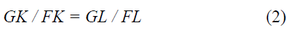
Where Lx and Ln are workforce employed in the relevant section and Kx and Kn are Capital
reserves in the relevant section. If will be applied first and second order derivative, in this case
based on the Pareto optimum condition following equality is established in terms of productivity
divided by inputs L and K:
Considering the saving resulting from the high ratio of export production we can assume the
following function than the above:

Here d is the amount of savings rates. According to the function Y = X + N and considering a
number of assumptions and mathematical operations is extracted following models:
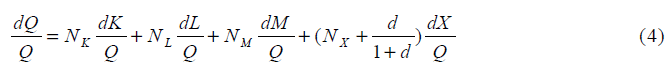
Where Nk = α is the marginal productivity of capital in the agricultural non-export sector, NL = β
is marginal productivity of labor in the agricultural non-export sector, NM = θ is marginal
productivity of import in the agricultural non-export sector and 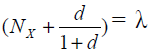 is the difference
between productivity and externality effect in the agricultural export sector. Thus on substituting
in Eq. (4) gives:
is the difference
between productivity and externality effect in the agricultural export sector. Thus on substituting
in Eq. (4) gives:
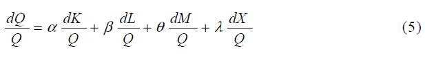
Eq. (5) is similar neoclassical function about economic growth. By employing Bruno [19]
statistical state solution assumption, Feder [17] sets the marginal sector products of labor equals
to the average labor product for the economy as a whole. Then one would arrive at the fairly
conventional growth equation by substitute NL = Ψ(Q/L) and dK = I into (5):
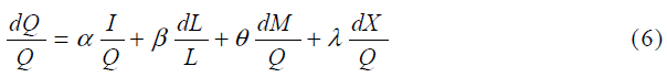
Indeed this equation can show the relationship between output growth, physical capital growth,
workforce growth and export growth in agricultural sector. The following modified Salehi [20]
model in logarithm form is used to examine the trade-growth nexus in agricultural sector in Iran.
The logarithm equation corresponding to Eq. (6) and breakdown of the factors agricultural sector
gives:

Where:
L(AVA) t is Logarithm of agricultural value added in 1997 constant prices based on million
dollars, L(IA) t is Logarithm of investment in agricultural sector in 1997 constant prices based on
million dollars, L(HA) t is Logarithm of human capital in agricultural sector based on thousands
(the number of employed workforce with a university degree), L(IMA)t is Logarithm of
agricultural imports in 1997 constant prices based on million dollars and L(EXA)t is Logarithm
of agricultural exports in 1997 constant prices based on million dollars.
Our empirical analysis in next Section is based on estimating directly long-run and short-run
variants of Eq. (7). All the data in this study are obtained from Central Bank of Iran (2004)1, the
Islamic Republic of Iran Customs Administration during the period 1961-2007.
The methodology
Recent advances in econometric literature dictate that the long run relation in Eq. (7) should
incorporate the short-run dynamic adjustment process. It is possible to achieve this aim by
expressing Eq. (7) in an error correction model as suggested by Engle and Granger [21]. Then,
the equation becomes as follows:
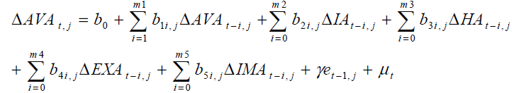 (8)
(8)
Where εt−1 is substituted by linear combination of the lagged variables as in Eq. (8):
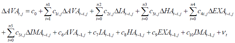 (9)
(9)
The long-run effect is measured by the estimates of lagged explanatory variables that are
normalized on estimate of c4. Once a long-run relationship has been established, Eq. (9) is
estimated using an appropriate lag selection criterion. At the second step of the ARDL cointegration
procedure, it is also possible to obtain the ARDL representation of the Error
Correction Model (ECM). To estimate the speed with which the dependent variable adjusts to
independent variables within the bounds testing approach, following Pesaran et al. [18] the
lagged level variables in Eq. (9) are replaced by ECt−1 as in Eq. (10):
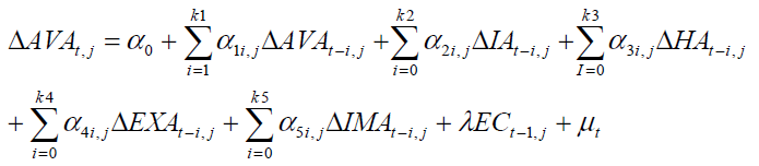 (10)
(10)
Methods such as Engel-Granger deal with small samples in non-validation studies because of
neglecting the short-term dynamic responses existing between variables. Also since Johansen-
Juselius tests are limitations on the condition stationary model variables, are used less than
ARDL test. However, one of the major disadvantages of ARDL test is that cannot show more
than one equilibrium relationship at estimation of model in unit it.
Results and Discussion
Unit Root Test
The model employed here is based on Perron [22] test, for the existence of unit root in a series,
which appears to be non-stationary. Accordingly, when structural break occurs, that may be
occur one of the following three conditions: 1) change of constant function of time trend, 2)
change of slope function of time trend, 3) change of constant and slope function of time trend.
According to these three cases, it is necessary to be estimated the following regression
relationship within the unit root test Perron [22]:

Where, Yt: Dependent variable, C: constant, T: trend, Y (-1): Y with one lag, TB: the time of
structural break, DU: dummy variable (if t > TB → DU=1 and The rest is zero years), DTB: if t= TB+1→ DTB=1 and the rest is zero years, DTt: trend dummy variable (if t > TB→ DTt=t-TB
and Zero for years before it). Based on given results of the Perron [22] model, the unit root null
hypothesis is rejected in favor of the alternative hypothesis if the t-statistic for ρ is greater than
the critical values tabulated by Perron [22]1. Under zero hypothesis (presence of unit root), tstatistics
related to Xt-1 coefficient (i.e. tβ) has limit distribution. The required critical values to
perform the test by Perron [22] are drawn and tabulated. These critical values regarding to λ
value show the ratio of structural break incidence time to the sample volume (λ=Tb/n).test
statistic related to other estimated coefficients has normal standard limit distribution when H0 is
rejected. Therefore, critical values of normal standard distribution can be used for significant
coefficients test. If t-statistic for β is bigger than the critical value tabulated by Perron [23], zero
hypotheses for the existence of unit root (non stationary) will be rejected. Results are given in Table 1.
Table 1: Results of Unit Root/ Stationary Test to determine structural break by Perron [22]
Based on the results reported in Table 1, the primary findings of the analysis are as follows. The
results of the Perron [22] model indicate that all series under investigation are non-stationary in
level and with one structural break function show strong evidence against the unit root
hypothesis in all of the variables under investigation except LIMA. The computed break dates
correspond closely with the expected dates associated with the effects of structural break in
1980, 1986, 1991 and 2002 and the effects of the drought in 1999. Under these circumstances
and especially when we are faced with mix results, applying the ARDL model is the efficient
way of the determining the long-run relationship among the variable under investigation.
Therefore, we will apply this methodology in the next section.
ARDL model
The empirical result based on ARDL tests repeated showed that the most significant break for
variables of under investigation are consistent with time of oil boom. Therefore, at this stage we
include four dummy variables; in order to take into account the structural breaks in the system.
The estimated coefficients of the long-run relationship and Error Correction Mode (ECM) are
displayed in Table 2.
Table 2: Estimated Long-run and ECM Coefficients using ARDL (1,0,0,0,0) Model
Table 2 shows that in the long run most coefficients are statistically significant and also, war
coefficient have a very significant effect on agricultural value added and increase in this
variables leads to decrease in agricultural value added. Alternatively, human capital in
agricultural sector does have an important effect on agricultural value added. In addition, the
coefficient of LHA in this model is statistically significant. It means that during the war,
employment has had negative growth rate and its share has declined while in these years’
employment growth rate in industrial and services sectors has climbed. Imports in agricultural
sector do have an important effect on agricultural value added. Since most exchange incomes are
obtained by oil incomes; consequently, increase in oil incomes has a good effect on imports
demand such that during oil boom period, just share of the consumed goods is increased out of
total imports and this is created due to increase in domestic demand resulted from consumption
in special levels of the society and insufficiency of domestic products to respond the created
demand overload.
As we see in Table 2, ECM version of this model show that the error correction coefficient
which determined speed of adjustment, had expected and significant negative sign. Bannerjee et
al. [24] holds that a highly significant error correction term is further proof of the existence of a
stable long-term relationship. The results indicated that deviation from the long-term in
inequality was corrected by approximately 42 percent over the following year or each year. This
means that the adjustment takes place relatively quickly, i.e. the speed of adjustment is relatively
high.
Diagnostic tests for serial correlation, normality, heteroscedasticity and functional form are
considered, and results are show that short-run model passes through all diagnostic tests in the
first stage. The results indicate that there is no evidence of Autocorrelation and that the model
passes the test for normality, and proving that the error term is normally distributed. Functional
form of model is well specified but there is existence of white heteroscedasticity in model. The
presence of heteroscedasticity does not affect the estimates and time series in the equation are of
mixed order of integration, i.e., I (0) and I (1), it is natural to detect heteroscedasticity.
These tests which have been proposed by Brown et al. [25] was tested the stability of model
coefficients. Its foundation is based on that initially, a regression equation including the variable desired is estimated using of estimated to be at least observations. Then, one observation is
added to the observations of previous equation and next estimation is performed and in this same
way, it is added to the observations a unit. In this way, after the estimation of each step, one
coefficient is obtained for any of the variables which finally is concluded a time series of
variables coefficients. These tests presents Cumulative sum (CUSUM) and cumulative sum of
Square (CUSUMSQ) diagrams between two straight lines (the bounds of the 95 percent).If the
diagram presented be within the boundaries, zero hypothesis is accepted which is based on lack
of structural break and if the diagram go out of the boundaries (it means that if dealt to them),
zero hypothesis is rejected which is based on lack of structural break and the presence of
structural break is accepted (Bahmani-Oskooee, [26]). CUSUM statistics is useful to find
systematic changes in long term coefficients of regression and CUSUMSQ statistics is helpful
when deviation from regression coefficients stability is randomized and occasional (short term).
According to Pesaran and Shin [27] the stability of the estimated coefficient of the error
correction model should also be empirically investigated. A graphical representation of CUSUM
and CUSUMSQ was shown in Figure 1. Following Bahmani-Oskooee [26] the null hypothesis (i.e.
that the regression equation is correctly specified) cannot be rejected if the plot of these statistics
remains within the critical bounds of the 5% significance level. As it is clear from Figure 1, the
plots of both the CUSUM and the CUSUMSQ are within the boundaries and hence these
statistics confirm the stability of the long run coefficients of regressors which affect the
inequality in the country. The stability of selected ARDL model specification is evaluated using
the cumulative sum (CUSUM) and the cumulative sum of squares (CUSUMSQ) of the recursive
residual test for the structural stability (see Brown et al., [25]). The model appears stable and
correctly specified given that neither the CUSUM nor the CUSUMSQ test statistics exceed the
bounds of the 5 percent level of significance.
Figure 1. Plots of CUSUM and CUSUMQ statistics for coefficients stability tests
Conclusion
This paper has provided a relationship between agricultural value added and human capital in
agricultural sector and also has explored the determinants of agricultural labor flows in Iran. In
this research at first we study variables Stationary and non-stationary by using from Phillips Perron, more than half of non-stationary variables with considering structural breaks show
Stationary process. Human capital coefficient in agricultural sector is positive and equal to 0.17
which shows that whit every percent increase in years of educated labor, agricultural value added
growth will increase by 0.17 percent. Therefore the analysis of the determinants of exit from
agricultural value added clearly shows that human capital plays a crucial role for agricultural
value added.
Consequently, one of the main and crucial factors in inefficiency is the improper utilization of
productive capacity in which we should also seek technologic changelessness in the country’s
production. Training is an important factor in human resources productivity improvement in
producing goods and services which causes growth. We should also mention that we should also
pay attention to training during work, vocational and technical trainings and public advanced
trainings; the last one is only limited to staff in Iran and has not been put into action yet. Since
human capital (educated sector) is the effective factors on GDP and also has a positive effect
with more time lag on GDP, so is recommended to reduce the time lag by improving quality of
workforce Training and implementing policies that lead to accelerating the positive effects of
human capital on GDP.
1National Accounts of Iran in 1997 constant prices
References
- Becker, B., Huselid, M. Res. Pers. Hum. Reso. Manag., 1998, 16, 53-101.
- Pacapaswiwat, S. Amarin Printing and Publishing Company, Bangkok, 2001.
- Desimone, R., Werner, J., Harris, D. Harc. Coll. Pub. Orl. FL, 2002.
- Yen, S. Amarin Printing and Publishing, Bangkok, 2008.
- Swanson, R., Holton, E. Berrett-Koehler Pub. Inc. San Francisco, 2001.
- Odusola, A. F. NES Proceedings. 1998.
- Burneth, N., Marble, K., Patrinos, H. A. Finance & Development, December 1995.
- Fishlow, A. Annual World Bank Conference on Development Economics, World Bank, 1995.
- Persson, T., Tabellins. Ame. Econ. Rev., 1994, 84, 600-621.
- Alesina, A., Dani, R. Q. J. Econ., 1994, 108: 465-90.
- Lucas, R. E. J. Mon. Econ, 1988, 22(1): 3-42.
- Lucas, R. E. B. Wor. Dev, 1993, 21(3): 391-406.
- Coulombe, S., Tremblay, J. F. J. Econ. Stu, 2001, 28(3): 154-180.
- Barro, R., Sala-i-Martin, X. Econ. Grow. McGraw-Hill, 1995.
- Stigliz, J. E. Annual World Bank Conference on Development Economics, 1998.
- Uwatt, B. U. NES Proceedings, 2002.
- Feder, G. J. Devel. Econ. 1982. 12:59-73.
- Pesaran, H. M., Shin, Y., Smith J. R. J. Appl. Econ., 2001, 16, 289–326.
- Bruno, M. Int. econ. Rev. 1968, 9(1):49-62.
- Salehi, Esfahani. H. Develop. Econ. 1991, 35:93-116.
- Engle R. F., Granger W. J. Econ. 1987, 55:251-276.
- Perron, P. Econ. 1989. 57:1361-1401.
- Perron, P. Econ. 1997. 80:355-385.
- Banerjee, A., Lumsdaine, R. L., Stock, J. H. J. Bus Econ. Statistics, 1992, 10: 271-287.
- Brown, R. L., Durbin, J., Evans, J. M. J. Royal. Statis. Society. 1975. 37:141-192.
- Bahmani-Oskooee, M. Japan and World Economy. 2001. 13:455-461.
- Pesaran, H. M., Shin, Y. The Ragnar Frisch Centennial Symposium (Cambridge: Cambridge University Press). 1999.
- Kankal, S. B., Gaikwad, R.W. Advances in Applied Science Research, 2011, 2 (1), 63.
- Elinge, C. M., Itodo, A. U., Peni, I. J., Birnin-Yauri, U. A., Mbongo, A. N. Advances in Applied Science Research, 2011, 2 (4), 279.
- Ameh, E. G., Akpah, F. A. Advances in Applied Science Research, 2011, 2 (1), 33.
- Ogbonna, O., Jimoh, W. L., Awagu, E. F., Bamishaiye, E. I. Advances in Applied Science Research, 2011, 2 (2), 62.
- Yadav, S. S., Kumar, R. Advances in Applied Science Research, 2011, 2 (2), 197.
- Sen, I., Shandil, A., Shrivastava, V. S. Advances in Applied Science Research, 2011, 2 (2), 161.
- Levine, D. M., Sulkin, S. D. J. Exp. Mar. Biol. Eco. 1984, 81: 211-223.
- Gupta N., Jain U. K. Der Pharmacia Sinica 2011 2(1):256:262.