Insights in Biomedicine Open Access

Keywords

Generalized Lindley distribution; Moments; Coefficient of variation; Skewness; Kurtosis; Index of dispersion; Lifetime data; Generalized gamma distribution; Goodness of fit

Introduction

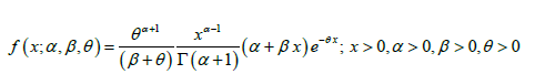
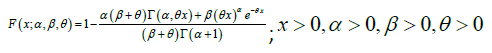
The probability density function of three-parameter generalized Lindley distribution (GLD) introduced by Zakerzadeh and Dolati (2009) having parameters α ,β ,and θ is given by:

(1.1)

Where

It is the complete gamma function.

It can be easily verified that the gamma distribution, the Lindley (1958) distribution and the exponential distribution are particular cases of (1.1) for (β = 0) , (α = β =1) and(α =1,β = 0) , respectively. Ghitany et al. have detailed study about various properties of Lindley distribution, estimation of parameter and application for modeling waiting time data in a bank. Detailed and comparative study on modeling of lifetime data using one parameter Lindley and exponential distributions [1].

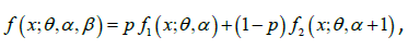
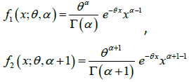
Further, the p.d.f. (1.1) can be easily expressed as a twocomponent mixture of gamma (α ,θ ) and gamma (α +1,θ ) distributions. We have,

(1.2)

where

,

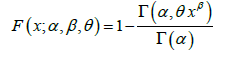
The corresponding distribution function of the GLD can be obtained as:

(1.3)

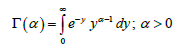
Where is the upper incomplete gamma function defined as:

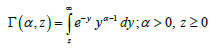(1.4)

The probability density function of three-parameter generalized gamma distribution (GGD) introduced by Stacy [2] having parameters α ,β ,and θis given by:

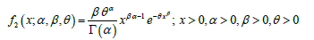(1.5)

Where α and β are the shape parameter and θ is the scale parameter. Clearly the gamma distribution, the Weibull distribution and the exponential distribution are particular cases of (3.1) for(β =1) , (α =1) and (α = β =1) respectively. Detailed discussion about GGD is available in [2] and parametric estimation for the GGD is available in [3]. In fact, GGD is the power gamma distribution.

The cumulative distribution function of the GGD is thus obtained as:

(1.6)

Where is the upper incomplete gamma function defined in (1.4).

Some of properties of GLD including nature of its p.d.f for varying values of its parameters, distribution of the sums of GLD, stochastic ordering, maximum likelihood estimates of parameters, distribution of the bivariate cases, and applications for modeling lifetime data [4]. It seems that some of its important properties based on moments including coefficient of variation, skewness, kurtosis, and index of dispersion has not been studied. Further, expressions for survival function, hazard rate function and mean residual life function of the distribution have not been obtained. Finally, the goodness of fit of GLD with two- parameter gamma, Weibull and lognormal distributions and concluded that the GLD is competing with these two-parameter distributions [4]. In fact, GLD should have been compared with other three-parameter lifetime distributions to test its goodness of fit. Recently Shanker and Shukla have detailed and critical study about the modeling of lifetime data from various fields of knowledge using threeparameter GLD and GGD and concluded that in majority of data sets GGD gives better fit [5].

In the present paper, the moments and moments based expressions including expressions for coefficient of variation, skewness, kurtosis, and index of dispersion have been given. The expressions for survival function, hazard rate function and mean residual life function have been obtained. The goodness of fit of GLD has been compared with the goodness of fit obtained by GGD and found that GLD does not give satisfactory fit in all data sets.

Moments and Associated Measures

Using mixture representation (1.2), the r^th moment about origin of GLD (1.1) can be obtained as:

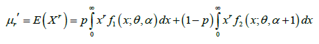
(2.1)

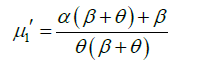
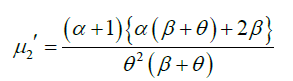
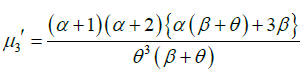
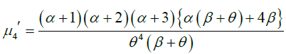
Substituting r =1,2,3, and 4 in (2.1), the first four moments about origin of GLD (1.1) are obtained as:

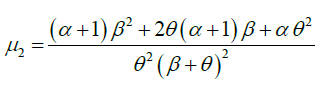
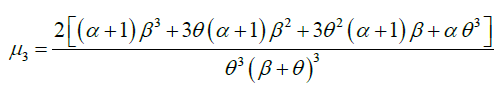
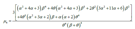
Again, using relationship between central moments and moments about origin, the central moments of GLD are obtained as:

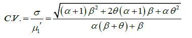
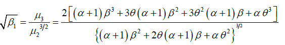
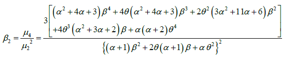
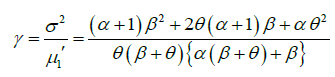
The expressions for coefficient of variation (C.V.) coefficient of skewness ,coefficient of kurtosis (β₂) , and index of dispersion (γ) of GLD are thus obtained as:

Hazard Rate Function and Mean Residual Life Function

Hazard rate function

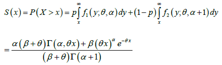
Using the mixture representation (1.2), the survival (reliability) function of GLD can be obtained as:

(3.1.1)

Where is the upper incomplete gamma function defined in (1.4).

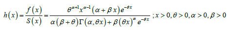
The hazard (or failure) rate function, h(x) of GLD is thus obtained as:

(3.1.2)

The shape of the hazard rate function, h(x) of the GLD is difficult to study because it includes the upper incomplete gamma function.

Mean residual life function

Using the mixture representation (1.2), the mean residual life function 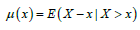of the GLD can be obtained as:

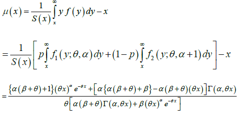
Where is the upper incomplete gamma function defined in (1.4).

The shape of the mean residual life function, μ(x) of the GLD is difficult to study because it includes the upper incomplete gamma function.

Maximum Likelihood Estimation

Maximum likelihood estimate (MLE) of GLD

Let 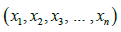be a random sample of size n from GLD (1.1). The likelihood function, L of GLD is given by

being the sample mean

The natural log likelihood function is thus obtained as:

The MLE of parameters θ , α ,β of GLD can be obtained by solving the natural log likelihood equation using R software (Package Stat 4).

Maximum likelihood estimate (MlE) of GGD

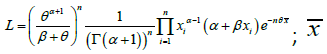
Assuming a random sample of size n from GGD (1.5), the likelihood function, L of GGD can be given as

being the sample mean.

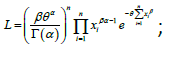
The natural log likelihood function is thus obtained as:

The MLE of parameters θ , α ,β of GGD can be obtained by solving the natural log likelihood equation using R software (Package Stat 4).

Applications and Goodness of Fit

In this section, the applications and goodness of fit of the GLD have been discussed for several lifetime data from biomedical science and engineering and the fit is compared GGD. The following eight lifetime data sets have been considered for testing the goodness of fit of GLD and GGD.

Data set 1

This data set used by Bhaumik et al. is vinyl chloride data obtained from clean up gradient monitoring wells in mg/l [6]:

Data set 2

This data set represents the waiting times (in minutes) before service of 100 Bank customers and examined and analyzed by Ghitany et al. [7] for fitting the Lindley distribution [8].

Data Set 3

This data is for the times between successive failures of air conditioning equipment in a Boeing 720 airplane [9].

Data set 4

This data set represents the lifetime’s data relating to relief times (in minutes) of 20 patients receiving an analgesic [10].

Data set 5

This data set is the strength data of glass of the aircraft window reported by [11].

Data set 6

The following data represent the tensile strength, measured in GPa, of 69 carbon fibers tested under tension at gauge lengths of 20 mm [12].

Data set 7

The following data set represents the failure times (in minutes) for a sample of 15 electronic components in an accelerated life test [13].

Data set 8

The following data set represents the number of cycles to failure for 25 100-cm specimens of yarn, tested at a particular strain level [13,14].

In order to compare the goodness of fit of GLD and GGD, values of −2ln L , K-S Statistics ( Kolmogorov-Smirnov Statistics) and p-values for the above data sets have been computed and presented in Table 1. The formulae for computing K-S Statistics are as follows:

	Model	ML Estimates			–2ln L	K-S Statistic	P-value
Data 1	GLD	1.0628	0.0006	0.5647	110.826	0.936	0.000
	GGD	5.9538	0.3802	5.2747	109.721	0.927	0.000
Data 2	GLD	2.0093	0.0007	0.2038	634.600	0.043	0.994
	GGD	3.8037	0.7017	0.8028	634.035	0.036	0.999
Data 3	GLD	0.9427	0.0003	0.0081	173.873	0.726	0.000
	GGD	26.6637	0.1736	12.7036	170.488	0.726	0.000
Data 4	GLD	9.6686	0.0029	5.0891	35.637	0.609	0.000
	GGD	51.4619	0.4350	39.4639	34.376	0.600	0.000
Data 5	GLD	17.9881	14.6111	0.6150	208.233	0.135	0.580
	GGD	19.6720	0.9814	0.6800	208.225	0.136	0.562
Data 6	GLD	22.7198	4.7710	9.3907	101.959	0.056	0.979
	GGD	3.5861	2.6483	0.3044	100.581	0.044	0.999
Data 7	GLD	1.2025	0.0832	0.0641	128.161	0.095	0.997
	GGD	0.8597	1.4152	0.0068	127.931	0.095	0.997
Data 8	GLD	0.8186	3.9740	0.0101	304.883	0.132	0.769
	GGD	1.9916	0.9426	0.0152	304.928	0.139	0.719

Table 1: ML Estimates, -2ln L, K-S Statistics and p-values of the fitted distributions of data sets 1 to 8.

Where k = the number of parameters, n = the sample size and is the empirical distribution function. The best distribution corresponds to lower values of −2ln L and K-S statistics and higher p- value.

It is obvious from the fitting of GLD and GGD that both are competing. But in data sets 5 and 8, GLD gives better fit than GGD and in all other data sets GGD gives better fit than GLD. It should be noted that [4] have considered data sets 7 and 8 for testing the goodness of fit of GLD and compared it with two - parameter gamma, Weibull and Lognormal distributions and concluded that GLD gives slightly better fit than these distributions.

Conclusion

In this paper moments and moments based characteristics including expressions for coefficient of variation, skewness, kurtosis and index of dispersion of the three-parameter generalized Lindley distribution (GLD) introduced by [4] have been derived and discussed. The expressions for the hazard rate function and the mean residual life function of the distribution have been obtained. The applications and goodness of fit of the distribution have been discussed with several lifetime data sets and the fit has been compared with the three –parameter generalized gamma distribution (GGD). The goodness of fit of the GLD and GGD shows that GGD gives better fit in majority of lifetime data sets and hence GGD can be considered as an important model over GLD for modeling lifetime data from biomedical science and engineering.

Acknowledgement

The author expresses his thankfulness the editor-in-chief and anonymous reviewers for their constructive comments which improved the quality of the paper.

References

1. Shanker R, Hagos F, Sujatha S (2015) On modeling of lifetimes data using exponential and Lindley distributions. Biometrics & Biostatistics International Journal 2(5): 1-9.
2. Stacy EW (1962) A generalization of the gamma distribution, Annals of Mathematical Statistics 33: 1187–1192.
3. Stacy EW,Mihram GA (1965) Parametric estimation for a generalized gamma distribution. Technometrics 7: 349-358.
4. Zakerzadeh H, Dolati A (2009) Generalized Lindley distribution, Journal of Mathematical extension 3(2):13–25.
5. Shanker R, Shukla KK (2016) On modeling of lifetime data using three parameters generalized Lindley and generalized gamma distributions. Biometrics & Biostatistics International Journal.
6. Bhaumik DK, Kapur K, Gibbons RD (2009) Testing parameters of a gamma distribution for small samples. Technometrics 51: 326-334.
7. Ghitany ME, Atieh B, Nadarajah S (2008) Lindley distribution and its Application. Mathematics Computing and Simulation 78: 493-506.
8. Lindley DV (1958)Fiducial distributions and Bayes’ theorem. Journal of the Royal Statistical Society. Series B 20: 102–107.
9. Proschan F (1963) Theoretical explanation of observed decreasing failure rate.Technometrics 5: 375-383.
10. Gross AJ, Clark VA (1975) Survival distributions: Reliability applications in the biometrical sciences. John Wiley, New York, USA.
11. Fuller EJ, Frieman S, Quinn J, Quinn G, Carter W (1994) Fracture mechanics approach to the design of glass aircraft windows: A case study. SPIE Proc 2286: 419-430.
12. Bader MG, Priest AM (1982) Statistical aspects of fiber and bundle strength in hybrid composites. In:Progressing Science in Engineering Composites. Tokyo, Japan.
13. Lawless JF (2003) Statistical models and methods for lifetime data. John Wiley and Sons, New York, USA.
14. Smith RL, Naylor JC (1987) A comparison of maximum likelihood and Bayesian estimators for the three parameter Weibull distribution. Applied Statistics 36: 358-369.