Research Article - (2023) Volume 10, Issue 1
Impact of Microfinance Credit Access on Households Income and Welfare: Evidence from Ethiopia
Asmamaw Getnet Wassie*
Department of Economics, Debre Tabor University, Debra Tabor, Ethiopia
*Correspondence:
Asmamaw Getnet Wassie,
Department of Economics, Debre Tabor University, Debra Tabor,
Ethiopia,
Email:
Received: 07-Nov-2022, Manuscript No. IPBJR-22-14680;
Editor assigned: 09-Nov-2022, Pre QC No. IPBJR-22-14680 (PQ);
Reviewed: 23-Nov-2022, QC No. IPBJR-22-14680;
Revised: 09-Jan-2023, Manuscript No. IPBJR-22-14680 (R);
Published:
16-Jan-2023, DOI: 10.21767/2394-3718-10.1.10
Abstract
Introduction: Welfare is the measure of the living standard of the society, and it is the other dimension of poverty. World has different groups of population in terms of living standards. Some of world’s population has been lived in luxuries house with many rooms. Hover, seven million people have been lived under extreme poverty. Above 40% of world population could not obtain $2 per day. The other recent studies indicate that about 900 million individuals in the world live in acute poverty based on income measurement of poverty. This indicates that poverty is at its high level all over the world but its concentration is very high at Sub Saharan Africa and South Asia.
Objective of the study: The main objective of this study is investigating the impact of microfinance credit access on households’ income and welfare case study in rural South Gondar.
Materials and methods: The study has used both inferential statistics and econometric model. Under the inferential section, the study has compared the socioeconomic characteristics of treatment group and controlled group in terms of mean, variance and T-test. The econometric part of the study has employed Propensity Score Matching method (PSM) of analysis. Limited dependent variable models are appropriate for PSM analysis to estimate the propensity score of treatment and control group.
Results and discussion: Sex of the respondent is one of the demographic variables that is employed by this study. Most of the respondents of the study were males (77.01%) but 22.99% were females. The mean age of females and males is 43 and 49 respectively. The mean income of females and males is 44912 and 57253 respectively. Even if the study did not test statistically, the average consumption of female headed and men headed households approximately same.
Conclusion: This study has examined the impact of credit access on households’ poverty reduction in terms of income and welfare case study in ACSI, rural South Gondar zone. The grand objective of the study is analyzing the impact of ACSI credit access on households’ income and welfare. The study has estimated the average treatment effect of credit access of ACSI on the borrowers (ATT) in terms of income and consumption. Since the nature of data in non-experimental, the study has used counterfactual.
Keywords
Inferential statistics; Econometric model; Propensity score; Independent variable
Identification
Introduction
Welfare is the measure of the living standard of the society,
and it is the other dimension of poverty. World has different
groups of population in terms of living standards. Some of
world’s population has been lived in luxuries house with many
rooms. Hover, seven million people have been lived under
extreme poverty. Above 40% of world population could not
obtain $2 per day. The other recent studies indicate that
about 900 million individuals in the world live in acute poverty
based on income measurement of poverty. This indicates that
poverty is at its high level all over the world but its
concentration is very high at Sub Saharan Africa and South
Asia. About 1.6 billion people are poor in terms of access to
social services and security. Ethiopia was the highest one in
the world where more than half of world’s population lives
below absolute poverty line in 2000. In case of Ethiopia 44%
of the total population was lived below poverty line.
Among different development programs, microcredit
institutions have succeeded in poverty reduction since 1970’s.
There are many supporters of microfinance for its positive
influence among clients of microcredit. In developing
economies formal financial institutions have ignored poor
section of population. Formal financial institutions did not
provide credit, saving and insurance for poor. Microfinance
institutions have gained considerable attention for its ability
to improve household’s income and welfare, and it has been
used as technique for poverty reduction. The impact of
microfinance credit service is doubt full. This is because
financial sustainability of microfinance institution is
unbalanced. This means financial institutions should work for
sustainable financial service provision for poor. Regardless of
this approach, other organizations have used microfinance
institution to develop different services continuously to
overcome requirements of poor. However, there is other
argument which says that microfinance has not significant
effect in developing economy since microfinance support
informal activities that have not enough market demand as a
result its effect on households’ income and welfare is
negligible.
There are a few studies regarding to the impact of
microfinance credit services on household’s income and
welfare Ethiopia like Bisrat, Hussien, Guruswaym and Birhanu.
Bisrat and Paul had conducted study on the role of
microfinance in alleviating urban poverty case study in Jimma
town, Ethiopia. The target population was clients of three
microfinance that are active Jimma. 120 clients of
microfinance were randomly selected and used for their
analysis. They used before-after test method of analysis while
they examined the impact of microfinance in poverty
reduction. Their study measured poverty in terms of income,
employment creation, asset holding and saving. They found
that income of clients has increase significantly after households used the services of microfinance. This means the
poverty of individuals who used the services of microfinance
is decreased in terms of monetary approach. Employment
creation for those who join microfinance is significantly
increased according to their result. Having their strength,
their study has its own limitation in terms of methodology.
They have attempted to examine the impact of microfinance
credit access in poverty reduction by using before after
approach with the help of descriptive statistics. However,
impact studies need strong econometric investigation rather
than weak descriptive and inferential statistics. Descriptive
statistics couldn’t isolate the impact of microfinance credit
access on the dependent variable. There may be problem of
selection bias. The other study conducted regarding to the
role of microfinance on poverty reduction was in Tigray region
by Guruswamy. He had conducted study on the role of
microfinance on poverty alleviation case study in Tigray,
Ethiopia. The main objective his study was assessing the role
of microfinance in reducing poverty in Tigray. Target
population for his study was the clients of DE Debit Credit and
Saving Institution (DCSI) who live in Mekellle. The method of
analysis employed by his study was more qualitative approach
and simple descriptive statistics. His analysis was focused on
households’ socioeconomic situations rather than on effect of
microfinance on poverty reduction. He found that
microfinance has positive on the life of individuals but he
found that the problems of DCSI while it provides its services
are high interest rate, loan application procedure, collateral
and lack of follow up. His study failed to show the role of
microfinance on poverty reduction with strong method of
analysis investigated the causality between micro-finance and
poverty in Ethiopia case study in Dale woreda in Sidama zone.
His study population was clients of Omo Microfinance
Institution (OMI). Two stage sampling procedure was used to
bring the representatives of the population. The total
numbers of sampling units were 200 who used for his study
analysis. He used both qualitative and quantitative methods
that are framed evaluative research approach. His study
attempted to measure poverty in terms of income of clients,
health and educational expenditures of households who are
clients of OMI. This means he attempted to investigate the
probable effect of microfinance on clients’ income, education
and expenditures. He found that client’s income has increased
after they are user of services of microfinance. According to
his result 52% of respondents had income in the range of
1000 birr-2000 birr. However, after they have the opportunity
of microfinance individuals’ income increases to the range
2001-3000. His study regression result failed to support the
significant effect of credits from microfinance to increase
income and health care of client sat 5% significance level.
Again, he found that the effect of microfinance credit on
access to education is insignificant. His study has its own
strong side even if again he has failed to use good impact
analysis model. His findings have not consistence. This means
from his inferential statistics he reported that microfinance increase income, access to education and health care of
clients. However, his simple econometric regression failed to
support findings from inferential statistics.
Among the mentioned studies on the above, no one had
conducted study on the impact of ACSI credit access on
income and welfare with the propensity score matching. All of
them had investigated the role of other microfinance
institutions in reducing poverty in terms of income and asset,
and some of the mentioned studies have methodological
limitation since they applied simple descriptive statistics.
However, impact evaluation studies with descriptive and weak
econometric models could not convey reliable information.
The most popular method of impact evaluation is Propensity
Score Matching (PSM). Having the above gaps, this study
examined the impact of ACSI credit access on households’
income and welfare using Propensity Score Matching method
(PSM) case study in the rural part of South Gondar, Ethiopia
[1-8].
Objective of the Study
The main objective of this study is investigating the impact of
microfinance credit access on households’ income and
welfare case study in rural South Gondar.
Specific Objective
In line with the general objective, the study has addressed the
following specific objectives.
• To examine the role of microfinance credit access on
borrowers’ income and welfare.
• To identify the main determinants of households’ decision
to participate in microfinance credit access.
Research Questions
The study has answered the following questions:
• What is the role of microfinance credit access on
borrowers’ income and welfare?
• What are the main determinants to participate in
microfinance credit access?
Materials and Methods
Description of the Study Area
The study is conducted in rural South Gondar zone where is
one of zonal administration of Amhara regional
administration. South Gondar is bordered with West Gojjam
on the South, West Gojjam with South West and Bahir Dar,
Lake Tana on the West and North Gondar on the North, Wage
hemra on the North East, North Wolo on the East, and North
Wolo on South East. South Gondar has different agro
ecological zones. These different agro ecological zones
provide good potential to agricultural activities in the study
area. The dominant economic activity that captures many
labor forces of the zone is agricultural sector. Based on the census projected by CSA, the total estimated population was
2,051,738.
Nature of Data and Sampling
In this study cross sectional data was employed to achieve the
objective of the study. Both qualitative and quantitative data
were employed. The population of the study was rural
households who live permanently in rural South Gondar,
Ethiopia. The study has applied multi stage sampling to draw
the representative households. First, the study stratified the
total population into different segment based on
administrative woreda. Second, the study selects four
woredas Farta woreda, Libokemkem woreda, Sidama Woreda
and Fogera woreda. Third, the study categorized households
into credit takers (treatment group) and noncredit takers
(controlled group). Finally, the study has selected kebeles
randomly in the selected woredas. According to 2013
population projection of CSA the total number household
heads in the four woredas was 225631. The study used
Yamane sample size determination cited in that is:
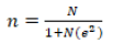
Where;
n=Sample size
N=Total household
E=Level of precision
Then, the study determined number of sample in each
selected woreda given its respective proportion:
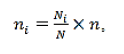
Where, Ni=Households in each selected woreda, i 1, 2, 3 and 4
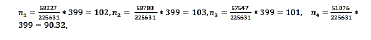
Where;
n1=Sample households in Farta woreda;
n2=Sample households in Fogera woreda;
n3=Sample households in Sidama woreda;
n4=Sample households in Libokemkem woreda.
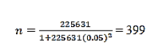
Hence, the study has statistically determined 399 households
for the analysis purpose. However, the study used additional
5% of statistically determined sample size since impact model
analysis requires large sample size so that 422 households
were used for unit of analysis. Half of the total sample was drawn from those individuals who had not taken credit from
ACSI but the remaining half was drawn from those who have
taken credit in ACSI.
This study has collected socioeconomic characteristics of the
sample by using structured questionnaires. Relevant data for
this study was collected from two groups that would be
categorized in to individuals who had not taken credit and
have taken credit in ACSI. This is because the study is aimed to
examine the impact of microfinance credit access on income
and welfare.
Method of Data Analysis and Model Specification
The study has used both inferential statistics and econometric
model. Under the inferential section, the study has compared
the socioeconomic characteristics of treatment group and
controlled group in terms of mean, variance and T-test. The
econometric part of the study has employed Propensity Score
Matching method (PSM) of analysis. Limited dependent
variable models are appropriate for PSM analysis to estimate
the propensity score of treatment and control group. The
most practical models of categorical outcome are binomial
and multinomial models which require the maximum
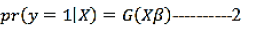
likelihood estimation to estimate the parameters. For Binary
outcome dependent variable let say y could take one of the
two possible outcomes. Logit and Probity are the most
probabilistic functional form of categorical outcome. The logit
regression model experience only dependent variable in
which it has only two values either 1 or 0. Logistic model has
assumed set of independent variables that would have an
effect on the dependent variable have logistic distribution.
Most econometrician and statisticians has appreciated the
underlying distribution assumption of independent variables
and error terms since most situations are not behave in
normal distribution. This study has used logistic model to
examine the determinants of the dependent variable of the
study.

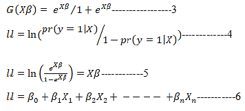
Where;
y is dependent variable,
Xi is set of independent variables for more compact
representation
Where;
X is vector of independent variable,
β is vectore of parameters.
We can write logistic function
Propensity Score Matching
Propensity score matching is techniques that solve the
problem of selection bias while we calculate the impact of a
given intervention. Observational studies are vulnerable to
bias when we estimate the causal inference of a certain
intervention. However, propensity score matching is the
panacea of such kind of problem by using counterfactual
techniques. The modern economy has applied different
interventions or programs to achieve a certain economic
objective. The effect of this intervention must be evaluated
with right technique. According to Alex et al., recent method
of matching is popular to evaluate the impact of intervention.
The propensity score matching method of evaluation drawn
the sample based on the observable characteristics of the
respondents. The propensity score matching method finds
matches of the treatment unit in the control unit given the
covariates. The matching process searches individual in the
control group who have same characteristics in the treatment
group. Propensity score matching method of evaluation of a
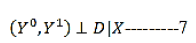
certain intervention has depends on two basic assumptions.
These assumptions are Conditional Independence (CIA)/
strong ignorability and common support. The conditional
independence assumptions states that the treatment variable
(D) assignment and the outcome variable (Y) are
independent each other.
The other assumption is common support. This assumption
states that a unit in the treatment group and respective
individual in the control have same propensity during the
assignment of treatment given the covariates (X). This
means that every unit in the treatment group (D=1)
must have corresponding unit with same probability P(X) in
the control group (D=0).

The common support assumption ensures that the covariates
not to predictor of the potential outcome. The matching of
treated unit and control unit is processed in the area where
there is overlap. The central objective of evaluation of a
certain intervention is estimation of the aggregate effect of
the program on the treatment group. Basically, there are two
types of aggregate effects of the intervention. These are
average treatment effect on the treated group (ATT). Average
treatment effect on the treated group (ATT) is the average impact on those individuals who have been exposed to the
program.

The average treatment effect on the treated group for the
sample is calculated as follow as:
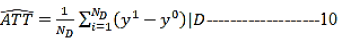
Where,
ND sample size of control group.
Average treatment effect on the treated group (ATT) is the
average advantage of the intervention to treat group who
drawn randomly from the treatment group. The other
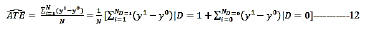
aggregate effect Average Treatment Effect (ATE). Average
Treatment Effect (ATE) is the average effect of the
intervention on the entire population for both treated and
control.

Where, Pr (D=1) and Pr (D=0) the probability of an individual
to involve in the intervention to treatment and control group
respectively. ATE to the sample
Matching of Covariates
In case of observational studies, the matching of covariates is
the best technique to isolate the effect of covariates on the
outcome of the intervention between treated and control
group. The central point of matching of covariates is creating
comparison group to treatment group given the covariates of
the model. Matching of covariates is non-experimental
approach. Propensity score is used to match covariates
between treatment and control group. There are different
matching methods like nearest-neighbor matching, Caliper
matching, Kernel and local linear matching.
Treatment and Outcome Variable
The treatment variable (D) of this study is the ACSI credit
access to households. The treatment variable (D) takes the
value 1 (D=1) if the individual takes credit in ACSI
otherwise 0 (D=0). The outcome variable of this study is
income and welfare of households in the rural part of South
Gondar.
Independent Variable Identification
The covariates of the model that are employed in this study
are sex of the household, marital status of the household, age
of the household, age square of the household, family size,
education status, agricultural land quality, agricultural land
availability, agricultural land size, and livestock ownership.
Sex of the household: It is obvious that sex is qualitative
variable. The studies assign value 1 if the household is male otherwise 0. The study has expected that sex has more
likelihood to access the ACSI credit. However, the study found
the reverse one. This means that being male has low
probability to take credit in ACSI relative to female headed
households.
Age of the household: Age is continuous variable in this
study. It is measured in years. The study has expected that as
younger households would have more likelihood to take
credit in ACSI. The logistic regression shows that younger
individuals have more likelihood to take credit in ACSI.
Age square of the household: The study has used the square
of age of households to account the probability of aged
households to access credit in ACSI. The study has expected
that aged households have less likelihood to take credit in
ACSI. The result supports this expectation. This means that
aged individuals have less likelihood to take credit in ACSI.
Marital status: Martial status has its own influence to take
credit. The nature of marital status is qualitative variable. For
this reason, the study assigned value 1 if the individual has
married, 0 otherwise. The study found that marital status has
negative and significant effect at 5% significance level. The
probability to take credit in ACSI will decrease with being
married relative to married households.
Family size: Family size is the member of individuals in a given
household. The study measured family size as continuous
variable. The study has expected that family size would have
positive and significant effect to take credit in ACSI. The result
shows that family size has insignificant effect.
Education: Households’ level of education is included in the
model of the study. The study measured education as
categorical variable. Even if the study expects positive effect
of higher education to access credit the result indicates that
education has not significant effect.
Agricultural land availability: Agricultural land is the major
resource of farmers. Therefore, farmers have considered their
land availability to decide to take credit and other economic
decisions. The study has designed agricultural land availability
as dummy variable to analysis purpose. The study found that
agricultural land availability has insignificant effect on the
dependent variable.
Agricultural land size: Agricultural land size also important
variable to farmers whether they decided to take credit or
not. That is the study has incorporated this variable in model.
In this study agricultural land size is measured as continuous
form of variable in hectare. The study has expected that
households who have higher agricultural land size would have
less probability to take credit relative to its counterpart.
However, it has insignificant effect.
Livestock ownership: Livestock ownership is also the other
variable that would have an effect on households’ decision to
take credit. The study has used Tropical Livestock Unit (TLU)
measurement to calculate livestock ownership of households.
The study has expected that as livestock ownership increases,
households would have less probability to take credit. The logistic regression indicates that livestock ownership has
positive and significant effect on the dependent variable.
Nature of the survey: The survey was administered for two
months between April and May in 2020. The survey was
conducted through face to face interview with structured
questionnaire. The survey was conducted in the rural South
Gondar, Ethiopia. The survey employed enumerators for
survey administers. The survey administers were trained for
two hours about how to present the questionnaire and
interview with respondents. Totally, survey administers were
four. All enumerators were BSc students. Respondents who
were employed in this study were household heads. The
study was proposed to survey 422 respondents. The study
was lucky in terms of response rate of the questionnaire since
the response rate was 100% [9-15].
Results and Discussion
Descriptive and Inferential Statistics
Characteristics of respondents over sex: Sex of the
respondent is one of the demographic variables that are employed by this study. Most of the respondents of the
study were males (77.01%) but 22.99% were females. The
mean age of females and males is 43 and 49 respectively.
The mean income of females and males is 44912
and 57253 respectively. Even if the study did not test
statistically, the average consumption of female headed and
men headed households approximately same. The mean
consumption of female headed and men household
headed households is 11078 and 11236 respectively.
Among 97 females of the respondents, 64.95% have taken
credit from ACSI. 46.46% of male respondents have taken
credit from ACSI (Tables 1 and 2).
| Sex |
Freq |
Percent |
Cum |
| Female |
97 |
22.99 |
22.99 |
| Male |
325 |
77.01 |
100 |
| Total |
422 |
100 |
|
Table 1: Sex of the respondent.
| Sex |
Treatment Var |
|
Total |
| Non-credit takers |
Credit takers |
| Female |
34 |
63 |
97 |
| Male |
174 |
151 |
325 |
| Total |
208 |
214 |
422 |
Table 2: Sex of the respondent and treatment variable.
Households’ Education Status
The study has categorized background of respondent’s
education into illiterate, attained formal education, and
attained informal education. 44.79%, 37.2% and 18.01% of
respondents had attained formal education, attained informal
education and had no attained any form of education
respectively. Most borrowers from ACSI are households who
attained formal education but the least borrowers are
households who had not attained any education (Tables 3
and 4).
| Education |
Freq |
Percent |
Cum |
| Illiterate |
76 |
18.01 |
18.01 |
| Formal |
189 |
44.79 |
62.8 |
| Informal |
157 |
37.2 |
100 |
| Total |
422 |
100 |
|
Table 3: Background of respondents’ education.
| Treatment Var |
Total |
| Education |
Non-credit takers |
Credit takers |
| Illiterate |
47 |
29 |
76 |
| Formal |
79 |
110 |
189 |
| Informal |
82 |
75 |
52 |
| Total |
208 |
214 |
422 |
Table 4: Background of respondent’s education and treatment variable.
Descriptive Statistics of Continuous Variable
The mean income, consumption, livestock, agricultural land
size, family size, and age of respondents are 54416.55, 11199.77, 4.637796, 6.190995, 4.729858, and 48.13981
respectively (Table 5).
| Variable |
Obs |
Mean |
Std. dev |
Min |
Max |
| Income |
422 |
54416.55 |
42906.37 |
1900 |
405000 |
| Consumption |
422 |
11199.77 |
7467.888 |
695 |
92970 |
| Livestock |
422 |
4.637796 |
1.644736 |
0 |
12.21 |
| Agricultural land size |
422 |
6.190995 |
3.204608 |
1 |
20 |
| Family size |
422 |
4.729858 |
2.231923 |
1 |
12 |
| Age |
422 |
48.13981 |
12.23976 |
20 |
85 |
Table 5: Summary of statistics of continuous variable.
Outcome and Treatment Variable
The treatment variable of the study is ACSI credit access, and
the outcome variables are income and consumption (Welfare)
of households. It is possible to describe the link between the
treatment variable and outcome variable by using T-Test. The
mean consumption to control group and treated group is
9255.1058 and 13089.902 respectively. The T-Test indicates
that there is significant difference between the consumption
of control group and treated group. The T-Test implies that
the average consumption of treated group is significantly
higher than the average consumption of the control group.
This implies that households who have taken credit from ACSI
have better welfare relative to households who have not
taken credit. However, the t-test of mean income between
treated and control group indicates that the average income
of control group is significantly higher than the average
income of treated group. This means that the access of credit
to households have not significant importance (Table 6).
| Variable |
Treatment group |
Control group |
Std. Err |
Confidence Interval |
| Mean |
Mean |
Treatment group |
Control group |
Treatment group |
Control group |
| Age |
46.61215 |
49.71154 |
0.756827 |
0.913744 |
(45.12 48.09) |
(47.91 51.50) |
| Family size |
4.443925 |
5.024038 |
0.149504 |
0.155633 |
(4.15 4.73) |
(4.71 5.32) |
| Agricultural land size |
5.957944 |
6.430769 |
0.22505 |
0.215054 |
(5.516.40) |
(6.00 6.85) |
| Income |
44043.2 |
65089.14 |
1571.67 |
3781.619 |
(40953 47132) |
(57655 72522) |
| Consumption |
13089.9 |
9255.106 |
429.1862 |
560.6044 |
(12246 13933) |
(8153 10357) |
| Livestock |
4.467196 |
4.813317 |
0.111906 |
0.113578 |
(4.24 4.68) |
(4.59 5.03) |
Table 6: Comparison of treatment and control group over continuous variable.
As the below tables shows, the mean average of continuous
variables in the control group is higher than the mean average of continuous variable in treatment group except
consumption (Tables 7 and 8).
| Group |
Freq |
Mean |
Std. err |
Std. dev |
95% CI |
| Control |
208 |
9255.106 |
560.6044 |
8085.151 |
8149.88 10360.33 |
| Treated |
214 |
13089.9 |
429.1862 |
6278.453 |
12243.91 13935.9 |
Note: Mean difference: -3834.796
H0: mean diff = 0; Ha: mean diff<0; Ha: mean diff ≠ 0; Ha: mean diff>0
PR (T<t)=0.0000; Pr (|T|>|t|)=0.0000; Pr(T>t)=1.0000
DF=420
T=-5.4507
Table 7: Household consumption difference over treatment variable.
| Group |
Freq |
Mean |
Std. err |
Std. dev |
95% CI |
| Control |
208 |
65089.14 |
3781.619 |
54539.29 |
57633.71 72544.57 |
| Treated |
2014 |
44043.2 |
1571.67 |
22991.55 |
40945.18 47141.22 |
Note: Mean difference: 21045.94
H0: mean diff = 0; Ha: mean diff<0; Ha: mean diff ≠ 0; Ha: mean diff>0
PR (T<t)=1.0000; Pr (|T|>|t|)=0.0000; Pr(T>t) = 0.0000
DF=420
T=-5.1905
Table 8: Household income difference over treatment variable.
Econometric Result
Logit model result: The study has conducted logistic
regression to identify factors that affect the household’s
likelihood to access credit in ACSI. Based on this result age,
age square, marital status, agricultural land availability, and
livestock ownership have significant effect on the households’
chance to access credit in ACSI. Sex, age square, marital
status, agricultural land availability, and livestock ownership
have negative and significant effect on the households’
likelihood to access credit in ACSI. The probability to take
credit in ACSI will decrease with being male relative to female
households.
This means that male headed households have lower chance
to take credit in ACSI relative to female headed households.
The other demographic variable that is included in the model
is age square of households. As the age of household
becomes high, the probability to take credit in ACSI will
decrease by 0.0004. Marital status of the household also
incorporated in the model, and it has negative and significant
effect at 5% significance level on the likelihood of households
to take credit in ACSI. Households who have married have
lower chance to take credit in ACSI relative to their
counterpart. Among economic variables that are included in
the model agricultural land availability and livestock
ownership have negative and significant effect at 10% and 5%
significance level on the dependent variable of the study.
Households who have agricultural land have lower chance to
take credit in ACSI relative to its counterpart. This is because
households who have agricultural land will not have demand
to credit relative to individuals who have not agricultural land.
With regarding to livestock, as household’s livestock increases
by a unit the probability to take credit in ACSI will decrease by
0.032. The background of household education has insignificant. However, age has positive and significant effect
at 1% significance level on the probability of the household to take credit in ACSI. The probability to take credit in
ACSI will increase as the household is younger (Table 9).
| Variable |
Coefficient |
P-value |
dy/dx |
p-value |
| Sex |
-0.709 |
0.007 |
-0.174 |
0.005 |
| -0.263 |
-0.062 |
| Age |
0.19 |
0.005 |
0.047 |
0.005 |
| -0.067 |
-0.016 |
| Age square |
-0.001 |
0.004 |
-0.0004 |
0.004 |
| -0.0006 |
-0.00016 |
| Marital status |
-0.859 |
0.034 |
-0.214 |
-0.214 |
| (0.405) |
-0.101 |
-0.101 |
| Family size |
-0.074 |
0.378 |
-0.016 |
0.378 |
| -0.065 |
-0.018 |
| Education status |
0.047 |
0.751 |
0.011 |
0.751 |
| -0.15 |
-0.037 |
| Agricultural land quality |
(-0.177) |
0.274 |
-0.044 |
0.274 |
| -0.162 |
-0.04 |
| Agricultural land avail |
(-1.357) |
0.118 |
(-0.301) |
0.043 |
| -0.867 |
-0.149 |
| Agricultural land size |
0.0381 |
0.432 |
0.008 |
0.432 |
| -0.032 |
-0.01 |
| Livestock |
(-0.131) |
0.064 |
(-0.032) |
0.064 |
| -0.071 |
-0.017 |
| Constant |
-1.654 |
0.589 |
|
|
| -0.894 |
Note: No of obs: 422; Pseudo R2: 0.0682; LR chi2(11): 39.89; log likelihood: -272.52092; Prob>chi2: 0.000
Table 9: Logistic regression and its marginal effect.
Propensity Score Estimation and Balancing Propensity
Score
The first step in impact evaluation using propensity score
matching is estimation of propensity score of the treatment
and control group over covariates. The dependent variable of
this study is binary that is households who have taken credit
in ACSI denoted by 1, otherwise 0 for households who have
not taken credit in ACSI. For this reason, the study has used
logistic model of regression to estimate the propensity score.
According to Horst et al., propensity score measures the
probability that an individual would be involved given the set
of covariates of the model. We can see the value of Pseudo R2 to say something about the balance of covariates of the
model between treatment group and control group after
matching the propensity score of the logistic regression.
Lower Pseudo R2 has facilitates to have good matching
between groups. Hence, this study is very lucky since its
Pseudo R2 is very low that is 0.015. We can use t-test to
confirm the balance of covariates between treatment group
and control group. The propensity score balanced test indicates that both treatment and controlled group have same
probability to access credit in ACSI given the covariates of the
model. It is also possible to see the distribution of propensity
score for treatment and control group before matching
(Figure 1 and Table 10).

Figure 1: Distributions of propensity score.
| Variable |
Mean |
Bias |
P-value |
| Treated |
Control |
| Sex |
0.71 |
0.64 |
13.5 |
0.216 |
| Age |
46.61 |
46.593 |
0.2 |
0.986 |
| Age square |
2294.7 |
2279.5 |
1.3 |
0.876 |
| Marital status |
0.83645 |
0.85514 |
-1.3 |
0.606 |
| Family size |
4.4439 |
4.4953 |
-2.3 |
0.804 |
| Education status |
1.215 |
1.2056 |
1.3 |
0.892 |
| Agricultural land avail |
0.93925 |
0.98131 |
-23 |
0.026 |
| Agricultural land size |
5.9579 |
6.3832 |
-13.3 |
0.163 |
| Agricultural land quality |
1.3925 |
1.3879 |
0.7 |
0.948 |
| Livestock |
4.4672 |
4.6 |
-8.1 |
0.406 |
Ps R2; LR chi2; Mean bias: 0.0159.016.5
Table 10: Test of propensity score between treatment and control group.
Matching Algorithm
Matching treatment and control group is the corner stone of
propensity score matching method. There are different
alternatives of matching methods that can match treated
units and control units given covariates. Criterions are
available to select the best matching method. According to
Dehejia and Wahba, balancing test, pseudo R2 and
large matched sample size are the criterion to choose
the best matching technique. In this study the best
matching algorithm is Kernel matching method with band
width 0.1 (Table 11).
| Matching methods size |
Balancing test |
Pseudo R2 |
Matched sample |
| Caliper (0.025) |
10 |
0.019 |
400 |
| Caliper (0.1) |
10 |
0.019 |
412 |
| Caliper (0.25) |
10 |
0.019 |
414 |
| Caliper (0.5) |
10 |
0.019 |
414 |
| NN (1) |
10 |
0.019 |
414 |
| NN (2) |
10 |
0.012 |
414 |
| NN (3) |
10 |
0.015 |
414 |
| NN (4) |
10 |
0.015 |
414 |
| NN (5) |
10 |
0.014 |
414 |
| Kernel (0.1) |
10 |
0.007 |
412 |
| Kernel (0.25) |
7 |
0.018 |
412 |
| Kernel (0.5) |
5 |
0.04 |
414 |
| Radius (0.1) |
4 |
0.051 |
414 |
| Radius (0.25) |
4 |
0.051 |
414 |
| Radius (0.5) |
4 |
0.051 |
414 |
Table 11: Choice of matching method.
Balance of Covariates after Matching
The study has checked the balance of covariates between
treated groups and control group before the choice of best
matching algorithm. However, testing balance of covariates
between the treatment group and control group before
matching is not that much feasible. Therefore, we have to test
the balance covariates between treatment and control group
after the choice of best matching method. The above table
shows that Kernel (0.1) is the best matching algorithm of this
study. The following table shows the balance of covariates
after matching. The balance of covariates after matching can
be verified by Pseudo R2, bias reduction, and probability
value. The Pseudo R2 must be low to have balanced covariates between treatment group and control group. In this study the
Pseudo R2 is very low after matching relative to unmatched
Pseudo R2. Pseudo R2 after matching is 0.007 but before
matching Pseudo R2 is 0.067. The other test of balance of
covariates is mean bias reduction. In this study the mean bias
before matching is 22% but mean bias after matching is
reduced to 4.2%. The other test is t-test or probability value.
In this test covariates must be insignificant after matching. In
this study eight covariates were not balanced between
treatment and control group before matching because
probability value is significant. However, after matching all
covariates are balanced between treatment and control group
because probability value is insignificant (Table 12).
| Variablele |
Unmatched/matched |
Mean |
Bias |
P-value |
| Treated |
Control |
| Sex |
Unmatched |
0.70561 |
0.83654 |
-31.5 |
0.001 |
| Matched |
0.72115 |
0.71899 |
0.5 |
0.961 |
| Age |
Unmatched |
46.612 |
49.712 |
-25.5 |
0.009 |
| Matched |
46.962 |
46.872 |
0.7 |
0.932 |
| Age square |
Unmatched |
2294.7 |
2644.1 |
-29.3 |
0.003 |
| Matched |
2325.8 |
2304.6 |
1.8 |
0.829 |
| Marital status |
Unmatched |
0.83645 |
1.0865 |
-17 |
0.08 |
| Matched |
0.85096 |
0.87105 |
-1.4 |
0.564 |
| Family size |
Unmatched |
4.4439 |
5.024 |
-26.2 |
0.007 |
| Matched |
4.5096 |
4.6811 |
-7.7 |
0.415 |
| Education |
Unmatched |
1.215 |
1.1683 |
6.5 |
0.505 |
| Matched |
1.2067 |
1.1986 |
1.1 |
0.908 |
| Agricultural land avail |
Unmatched |
0.93925 |
0.99038 |
-28 |
0.004 |
| Matched |
0.96635 |
0.98788 |
-11.8 |
57.9 |
| Agricultural land size |
Unmatched |
5.9579 |
6.4308 |
-14.8 |
0.13 |
| Matched |
6.1298 |
6.4332 |
-9.5 |
0.328 |
| Agricultural land quality |
Unmatched |
1.3925 |
1.5337 |
-19.7 |
0.043 |
| Matched |
1.4327 |
1.4181 |
2 |
0.839 |
| Livestock |
Unmatched |
4.4672 |
4.8133 |
-21.1 |
0.031 |
| Matched |
4.5325 |
4.6193 |
-5.3 |
0.566 |
Note: Sample: Pseudo R2 P; Unmatched: 0.06722.0; Matched: 0.0074.2
Table 12: Propensity score balancing test.
Estimation of Average Treatment Effect to Treated
Group (ATT)
Estimation of average treatment effect on the treated group is
the central point of impact studies in general and propensity
score matching in particular. According to Moreno-Serra, it
represents the average impact of the intervention on
individuals who exposed to a given intervention. Average
treatment effect to the treated group is the measure of the
average effect of the intervention on individuals who are
drawn randomly in the treated group. As the study mentioned
on its methodology the outcome variable of this study are
income and consumption. Therefore, this study has estimated
average treatment effect on the income and consumption of
the treated group. While the study estimated average
treatment effect on the treated group, eight numbers of
individuals have discarded in the treated group because these
eight individuals are off support of the common support. The
average treatment effect on the treated group (ATT) in terms
of income on the treated group is 44390.8981 but on control
group is 56884.9369. The difference of ATT in terms of income
between treated and control group is negative. However, the
average treatment effect (ATT) in terms of consumption on
the treated group is 13323.0874, and on the control group is
8920.84951. The difference is positive. This implies that credit
takers’ welfare that is measured by consumption is improved.
However, estimation of average treatment effect to treatment
group is not that much relevant without the best matching
algorithm. This is because without correct matching it is
difficult to separate the effect of the intervention effect on
the outcome variable. The average treatment effect on the
treatment group (ATT) in terms of income is 44409.2548
which is less than ATT of control group that is 58895.7629.
This may be due to the problem of households’ credit
allocation in productive activity after they have taken credit.
Households may spend the credit in the area of unproductive
investment. However, average treatment effect on the
treatment group (ATT) in terms of consumption is 13198.9375
which are higher than ATT of control group that is
9989.14274. This implies that ACSI credit access has improved
the welfare of households in terms of consumption. This
means ACSI credit access has reduced poverty of households
in terms of poverty [16-20] (Tables 13-16).
| Psmacth 2: Treatment assignment |
Psmatch 2: Common support |
Total |
| Off support |
On support |
| Untreated |
0 |
208 |
208 |
| Treated |
8 |
206 |
214 |
| Total |
8 |
414 |
422 |
Table 13: Common support before choice of matching method.
| Variable |
Sample |
Treated |
Control |
Difference |
S.E |
T-stat |
| Income |
Unmatched |
44043.2 |
65089.14 |
-21045.9 |
4054.665 |
-5.19 |
| ATT |
44390.9 |
56884.94 |
-12494 |
5338.084 |
-2.34 |
| Consumption |
Unmatched |
13089.9 |
9255.106 |
3834.796 |
703.5423 |
5.45 |
| ATT |
13323.09 |
8920.85 |
4402.238 |
802.5027 |
5.49 |
Table 14: ATT estimation before choice of matching method.
| Psmacth 2: Treatment assignment |
Psmatch 2: Common support |
Total |
| Off support |
On support |
| Untreated |
4 |
204 |
208 |
| Treated |
6 |
208 |
214 |
| Total |
10 |
412 |
422 |
Table 15: Common support after choice of matching method.
| Variable |
Sample |
Treated |
Control |
Difference |
S.E |
T-stat |
| Income |
Unmatched |
44043.2 |
65089.14 |
-21045.9 |
4054.665 |
-5.19 |
| ATT |
44409.25 |
58895.76 |
-14486.5 |
4670.088 |
-3.1 |
| Consumption |
Unmatched |
13089.9 |
9255.106 |
3834.796 |
703.5423 |
5.45 |
| ATT |
13198.94 |
9989.143 |
3209.795 |
781.9841 |
4.1 |
Table 16: ATT Estimation after choice of matching.
Conclusion
This study has examined the impact of credit access on
households’ poverty reduction in terms of income and
welfare case study in ACSI, rural South Gondar zone. The
grand objective of the study is analyzing the impact of ACSI
credit access on households’ income and welfare. The study
has estimated the average treatment effect of credit access of
ACSI on the borrowers (ATT) in terms of income and
consumption. Since the nature of data in non-experimental,
the study has used counterfactual. To have best matching
between treatment and control group, the study has tested
different matching methods like Kernel, Caliper, nearest
neighbor, and radius. The best matching method to this study
is kernel (0.1). The study found that the ATT on the treatment
group in terms of income is less than the control group. This
implies that the role of ACSI credit access did not increase the
income of borrowers. This may be due to that borrowers did
not allocate their credit in the productive economic activity.
However, The ATT of treatment group in terms of
consumption is higher than the controlled group. This implies
that the role of ACSI credit has improved the welfare of
borrowers.
Recommendations
The study has suggested the following recommendation to
responsible body regarding to the impact of microfinance on
household’s income and welfare.
• The estimation of ATT on the treated group in terms of
income is less than its counterpart. This finding is
somewhat surprising and the impact of microfinance on
households’ income is questionable. The expectation
regarding to the impact of microfinance on client
households’ income was higher relative to non-clients.
However, the finding is on the contrary. This may be due to
that borrowers would allocate the loan on unproductive
area of economic activity. Hence, the responsible body
should aware households who take credit to allocate their
credit on productive area of economic activity, and if it is
feasible and possible design follow up scheme that will
restrict the loan allocation that would be taken by
borrowers. In other word, government or microfinance
sector should follow borrowers’ loan allocation.
• Based on the estimation of ATT on the treated group in
terms of welfare, it is higher than the ATT of control group.
This implies that ACSI credit access has improved welfare of borrowers relative to non-borrowers. Therefore,
microfinance sector should continue its credit access to
households.
Funding Statement
This research did not receive any specific grant from funding
agencies in the public, commercial, or not-for-profit sectors.
Data Availability Statement
Data will be made available on request.
References
- Dehejia RH, Wahba S (2002) Propensity score-matching methods for nonexperimental causal studies. Rev Econ Stat. 84(1):151-161.
[Crossref] [Google Scholar]
- Guruswamy D (2012) The role of microfinance institutions on poverty alleviation in Ethiopia. Indian J Res Commer Manag. (1):9-16.
[Google Scholar]
- Heckman JJ (2010) Selection bias and self-selection. Econom. 1:1-2.
[Google Scholar]
- Horst SJ, Harris H, Horst SJ (2016) A brief guide to decisions at each step of the propensity score matching process. Pract Assess Res. 21(1-4):1-11.
[Google Scholar]
- Hussien M (2017) Causality between micro-finance and poverty in Ethiopia: An empirical investigation. Int J Adv Res. 7(1):1-4.
[Google Scholar]
- Kanbur R, and Squire L (1999) The evolution of thinking about poverty: Exploring the Interactions. Appl Econ Res. 9(1):13-14.
[Google Scholar]
- Mecha NS (2017) Effect of microfinance on poverty reduction: A critical scrutiny of theoretical literature. Glob J Manag Bus Res. 6(3):16-33.
- Serra MR (2007) Matching estimators of average treatment effects: A review applied to the evaluation of health care programmes. Centre for health economics, university of York publishing, Heslington, United Kingdom.
[Google Scholar]
- Scherer NF, Doany FE, Zewail AH, Perry JW (1986) Direct picosecond time resolution of unimolecular reactions initiated by local mode excitation. Chem Phys. 84(3):1932-1933.
[Google Scholar]
- Shepherd A (2007) Understanding and explaining chronic poverty An evolving framework for Phase III of CPRC’s research. CPRC working paper 80, Westminster bridge road London, UK. 1-41.
[Google Scholar]
- Sinha F (2006) Does the microfinance reduce poverty in India? Propensity score matching based on a national level household data. 17:1-31.
[Google Scholar]
- Tarekegn M (2018) The paradox of poverty reduction in Ethiopia: Are microfinance institutions the paradox of poverty reduction in Ethiopia: Are microfinance institutions really pro-poor ? 8(3):1-7.
[Google Scholar]
- Tarozzi A, Desai J, Johnson K (2015) The impacts of microcredit: Evidence from Ethiopia. 7(1):54-89.
[Google Scholar]
- Dehejia, RH, Wahba S (1998) Propensity score matching methods for non-experimental causal studies. Rev Econ Stat. 84(1):151-161.
[Crossref] [Google Scholar]
- Santoso DB, Gan C, Revindo MD, Massie NWG (2020) The impact of microfinance on Indonesian rural households' welfare. Agric Finance Rev. 80(4):491-506.
[Crossref] [Google Scholar]
- Mahmud S (2003) Actually how empowering is microcredit? Dev Change. 34(4):577-605.
[Crossref] [Google Scholar]
- Nghiem S, Coelli T, Rao P (2012) Assessing the welfare effects of microfinance in Vietnam: Empirical results from a quasi-experimental survey. J Dev Stud. 48(5):619-632.
[Crossref] [Google Scholar]
- Al-Shami SSA, Razali RM, Rashid N (2018) The effect of microcredit on women empowerment in welfare and decisions making in Malaysia. Soc Indic Res. 137(2):1073-1090.
[Google Scholar]
- Amin A, Hossain I, Mathbor GM (2013) Women empowerment through microcredit: Rhetoric or reality. An evidence from Bangladesh. Generos. 2(2):107-126.
[Google Scholar]
- Li X, Gan C, Hu B (2011) The impact of microcredit on women's empowerment: Evidence from China. J Chinese Econ Bus Stud 9(3):239-261.
[Crossref] [Google Scholar]
Citation: Wassie AG (2023) Impact of Microfinance Credit Access on Households Income and Welfare: Evidence from Ethiopia. Br J Res. 10:10.
Copyright: © 2023 Wassie AG. This is an open-access article distributed under the terms of the Creative Commons Attribution License, which permits unrestricted use, distribution, and reproduction in any medium, provided the original author and source are credited.