Journal of Heavy Metal Toxicity and Diseases Open Access

Keywords

Heavy metals; EDXRF; Sediments; Pollution indices; Tamil Nadu

Introduction

Human actions are causing the slow extermination of plant and animal species in nature through toxic pollution due to industrial and technological advancement in recent decades [1]. Heavy metals are both extremely toxic and ubiquitous in natural environments and they occur in soil, surface water and plants, and it is readily mobilized by human activities such as mining and dumping industrial waste in natural habitats such as forests, rivers, lakes, and ocean [2].

Heavy metal pollution is one of the environmental crises that accompany with the rapid economic development in many countries. For heavy metal pollutants, one of the largest problems associated with their threat to the ecosystem is the potential for bioaccumulation and biomagnifications causing heavier exposure for some organisms than is present in the environment alone [3]. Due to the toxicity and persistence of heavy metal pollution, heavy metal research of estuarine and coastal area has attracted more public concerns recently [4-9]. It is necessary to investigate the distribution and pollution degree of heavy metal, in order to interpret the mechanism of transportation and accumulation of pollutants and to provide basic information for coast utilization and supervision [10, 11].

Sediment quality has been recognized as an important indicator of water pollution since sediments are the main sink for various pollutants, including metals discharged into the environment [12- 17]. Sediments also play a significant role in the remobilization of contaminants in aquatic systems under favorable conditions and in interactions between water and sediment. Comprehensive methods for identifying and assessing the severity of sediment contamination have been introduced in order to protect the aquatic life community [18, 19]. Sediment analysis is vital to assessing qualities of total ecosystem of a water body in addition to water sample analysis practiced for many years. The EDXRF technique is chosen for the present work due to its advantages like non-requirement of chemical treatment of the samples; it is less time consuming non-destructive method and it is ideal for environmental research.

This paper reports the elemental concentrations of coastal sediments from Pattipulam to Dhevanampattinam of East Coast of Tamil Nadu, Bay of Bengal. This coast is a densely populated area with variety of industrial activities (such as metal smelting, pharmaceuticals, etc.) and agriculture activities (which include maize, cassava, sugarcane and vegetables farming). All these activities release toxic and potentially toxic metals to the environment. This research therefore aims at assessing the influence and sources of these toxic and potentially toxic metals on the sediments from East Coast of Tamil Nadu. The samples were subjected to geochemical analyses using EDXRF technique and to evaluate possible anthropogenic influences. The main objectives of the current study are: (1) to determine concentrations of metals exist in the sediments from Pattipulam to Dhevanampattinam of East Coast of Tamil Nadu and (2) assess the degree of contamination by heavy metals in sediments using pollution indices.

Materials and Methods

Sampling and sample preparation

Sediment samples were collected along the Bay of Bengal coastline, from Pattipulam to Devanampattinam coast during pre-monsoon condition. These samples were collected pre-monsoon season, when sediment texture and ecological conditions can be clearly observed, when erosional activities are predominant and sediments were not transported from the river and estuary towards the beach and marine. In order to ensure minimum disturbance of the upper layer, samples were collected by a Peterson grab sampler from 10 m water depths parallel to the shoreline. The grab sampler collects 10 cm thick bottom sediment layer from the seabed along the 22 stations. Sampling locations were selected to collect representative samples from all along the study area. Table 1 represents the geographical latitude and longitude for the sampling locations at the study area.

S. No.	Location ID	Latitude (N)	Longitude (E)	Location
1	PPM	12°40'51.27"N	80°15'19.35"E	Pattipulam
2	DVN	12°39'19.32"N	80°14'49.68"E	Devaneri
3	MAM	12°37'55.53"N	80°14'13.14"E	Mahabalipuram
4	KKM	12°34'56.33"N	80°13'22.37"E	Kokilamedu
5	KPM	12°30'57.52"N	80°11'50.57"E	Kalpakkam
6	VPC	12°27'58.97"N	80°11'16.29"E	Veppancheri
7	TPM	12°24'42.28"N	80° 9'48.29"E	Thenpattinam
8	MKM	12°21'26.51"N	80° 6'52.67"E	Mudaliyarkuppam
9	OKM	12°19'35.89"N	80° 5'44.70"E	Odiyurkuppam
10	APT	12°16'19.80"N	80° 3'16.00"E	Alampara fort
11	KPK	12°12'42.65"N	80° 1'32.40"E	Kaipanikuppam
12	FBH	12° 9'2.75"N	79°59'11.44"E	French beach
13	KMU	12° 4'59.37"N	79°55'53.55"E	Koonimedu
14	GCM	12° 2'45.84"N	79°56'46.86"E	Ganapathichettikulam
15	ABH	11°59'51.98"N	79°55'31.39"E	Auroville beach
16	MPT	11°57'43.22"N	79°52'42.65"E	Muthiyalpet
17	PBH	11°56'38.16"N	79°52'17.45"E	Pondy beach
18	KEP	11°54'23.61"N	79°51'49.37"E	Keerapalayam
19	PPT	11°52'45.44"N	79°51'19.75"E	Puthupettai
20	KIP	11°50'23.50"N	79°51'54.44"E	Kirumampakkam
21	TKA	11°46'28.21"N	79°49'31.03"E	Thazhankuda
22	DPM	11°44'41.37"N	79°49'23.01"E	Dhevanampattinam

Table 1: The Geographical latitude and longitude for the sampling locations.

The sampling locations were selected based on the prevailing stresses and included areas near the urban and domestic effluent discharge point. Uniform quantity of sediment samples were collected from all the sampling stations located between an average interval of 3 NM (Nautical mile). Each sample of about 2 kg was kept in a thick plastic bag. Care was taken to ensure that the collected sediments were not in contact with the metallic dredge of the sampler, and the top sediment layer was scooped with an acid washed plastic spatula. Sediment samples were stored in plastic bags and kept in refrigeration at -4ºC until analysis. Then pebbles, leaves and other foreign particles were removed. The samples were sub-sampled using the coning and quartering method.

The samples were air dried at 105ºC for 24 h to a constant weight and sieved using a 63 μm sievein order to identify the geochemical concentrations. The grain size <63 μm, which presents several advantages: (1) heavy metals are mainly linked to silt and clay; (2) this grain size is like that of the suspended matter in water; and (3) it has been used in many studies on heavymetal contamination. Then samples were ground into a fine powder for 10-15 min, using an agate martor. All powder samples were stored in desiccators until they were analyzed. One gram of the fine ground sample and 0.5 g of the boric acid (H₃BO₃) were mixed. The mixture was thoroughly ground and pressed to a pellet of 25 mm diameter using a hydraulic press (20 tons) [9]. The Figure 1 shows the sampling location of the Study area.

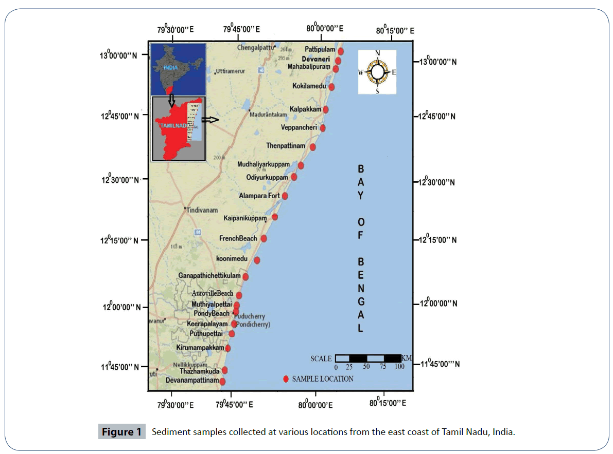
Figure 1 Sediment samples collected at various locations from the east coast of Tamil Nadu, India.

EDXRF technique

The prepared pellets were analysed using the EDXRF available at Environmental and Safety Division, Indira Gandhi Centre for Atomic Research (IGCAR), Kalpakkam, Tamilnadu. The instrument used for this study consists of an EDXRF spectrometer of model EX-6600SDD supplied by Xenemetrix, Israel. The spectrometer is fitted with a side window X-ray tube (370 W) that has Rhodium as anode. The power specifications of the tube are 3-60 kV; 10-5833 μA. Selection of filters, tube voltage, sample position and current are fully customizable. The detector SDD 25 mm2 has an energy resolution of 136 eV ± 5 eV at 5.9 keV Mn X-ray and 10 sample turret enables keeping and analysing 10 samples at a time. The quantitative analysis is carried out by the In-built software NEXT. A standard soil (NIST SRM 2709a) was used as reference material for standardizing the instrument. This soil standard obtained from a follow field in the central California San Joaquin valley. The soil standard (reference material) (NIST SRM 2709a) analysis value are given in Table 2.

Element	Certified Values	EDXRF values
Mg	14600	14900± 1000
Al	72100	68400±2300
K	20500	19100± 700
Ca	19100	16500± 500
Ti	3400	3100± 100
Fe	33600	33900±1200
V	110	98.8± 6.59
Cr	130	112.1± 4.01
Mn	529	568.2± 19.85
Co	12.8	12.8± 0.55
Ni	83	69.3± 2.98
Zn	107	127.9± 4.88

Table 2 Analysis of soil standard-NIST SRM 2709a by EDXRF (mg kg-1).

Results and Discussion

Heavy metals in sediments

The determined heavy metals in sediment samples by EDXRF technique given in Table 3. The mean concentration found to be : 1665 mg kg^-1 for Mg; 21719 mg kg^-1 for Al; 8405 mg kg^-1 for K; 9284 mg kg^-1 for Ca; 1520 mg kg^-1 for Ti; 6554 mg kg^-1 for Fe; 35.3 mg kg^-1 for V; 30.1 mg kg^-1 for Cr; 130.4 mg kg^-1 for Mn; 2.4 mg kg^-1 for Co; 20.2 mg kg^-1 for Ni; 62.2 mg kg^-1 for Zn, 6.2 mg kg^-1 for As, 3.4 mg kg^-1 for Cd; 404.9 mg kg^-1 for Ba; 15.1 mg kg^-1 for La; 12.1 mg kg^-1 for Pb; This mean concentration values of heavy metals in sediments do not exceed the natural background levels of heavy metals given by Turekian and Wedepohl [20]. This indicates that study area dominated with large amount of natural sediment with low heavy metal content [21]. The determined mean metal concentration is in the order of Al > Ca > K > Fe > Mg > Ti > Ba > Mn > Zn > V > Cr > Ni > La > Pb > As > Cd > Co.

S.No.	Location ID	Location	Mg	Al	K	Ca	Ti	Fe	V	Cr	Mn	Co	Ni	Zn	As	Cd	Ba	La	Pb
1	PPM	Pattipulam	500	21722	9200	8550	1043	5486	26.9	29.9	108.8	2.1	18	66	6.2	4.9	422.9	9.9	12.9
2	DVN	Devaneri	2600	27900	8900	11000	9889	21836	162.2	61.9	386.9	7.1	20.3	58.7	7	3.2	362.8	123	14
3	MAM	Mahabalipuram	900	21800	8300	9800	2122	9138	45.8	31.6	178.3	3.3	18.7	34.1	5.8	0	435.8	10.2	6.1
4	KKM	Kokilamedu	1500	24000	9300	10500	1911	7557	35.6	26.3	156.5	2.7	18.1	27.9	5.6	4.7	485.2	21.8	6.1
5	KPM	Kalpakkam	900	22600	9300	9500	1352	6396	30.5	28	120.5	2.1	18.6	36.2	5.7	3.9	434.4	20.4	10
6	VPC	Veppancheri	2500	24900	9000	9800	1614	7355	34.2	29.4	138.5	2.7	20	36.5	5.3	7.5	453.8	18.1	8.9
7	TPM	Thenpattinam	4200	23700	8700	10800	1543	7423	35.6	38.6	153.5	2.8	24	120.3	8.4	2.6	434.6	18.7	25.8
8	MKM	Mudaliyarkuppam	20	17700	7200	7000	779	3945	23.8	21.7	88.9	1.4	19.7	50.1	5.5	0	302.9	7.5	7
9	OKM	Odiyurkuppam	200	18300	8100	8100	661	4036	24	21.4	81.6	1.4	16.6	22.7	4.9	2.7	421.5	0	3.8
10	APT	Alampara fort	2400	23200	8600	10400	859	5513	28	23.6	113.2	2.1	20.6	44.2	5.5	4.6	436	2.4	7.3
11	KPK	Kaipanikuppam	600	17800	7400	6400	614	3532	23.2	19.2	77.2	1.2	16.3	34.9	4.7	5.2	348.9	6	2.3
12	FBH	French beach	2600	20200	7300	8500	1242	6283	29.5	27.8	136.5	2.3	19.3	34.9	4.7	7.1	335.4	4.8	4.5
13	KMU	Koonimedu	2500	21800	7900	9400	1089	5694	28.2	32.3	123.9	2.1	21.8	121.9	8.3	0.2	337.1	1.1	24.7
14	GCM	Ganapathichettikulam	1600	19900	7800	8100	845	4509	24.7	29.3	95.9	1.6	21.5	116.8	7.2	0	373.2	15.5	22.5
15	ABH	Auroville beach	1500	21700	9100	10400	1027	5431	26.1	26.7	109.2	2	18.3	44.2	5.6	4.8	426.8	12.7	7.5
16	MPT	Muthiyalpet	1600	21500	8900	9300	942	4866	25.3	24.6	103.1	1.7	24.3	66.3	6.7	0	402.5	6.9	14
17	PBH	Pondy beach	1300	22600	9300	9600	772	4649	24.9	25.9	95.1	1.8	25.8	83.8	6.7	2.5	442.4	10.8	18.6
18	KEP	Keerapalayam	1800	26100	9500	12500	753	5303	26.6	26.3	115.8	2	22.8	87.6	7	13.7	433.4	2.6	16.4
19	PPT	Puthupettai	1800	20000	8000	8400	945	5433	27.3	30.7	102	2.1	19.1	65.9	6.3	0	450.4	13.2	14.2
20	KIP	Kirumampakkam	2500	23100	7700	10700	1632	8982	36.9	40.7	184	3.3	21.4	53.8	5.5	3.7	373.9	2.4	9.6
21	TKA	Thazhankuda	1900	15800	7600	5800	376	3215	22.7	19.8	61.4	1.1	17.9	91.1	6.7	2.5	393.2	3	18.7
22	DPM	Dhevanampattinam	1200	21500	7800	9700	1422	7604	35	45.6	138.3	2.9	22.1	70.3	6.3	1.5	401.6	20.2	11.7
Mean			1665	21719	8405	9284	1520	6554	35.3	30.1	130.4	2.4	20.2	62.2	6.2	3.4	404.9	15.1	12.1

Table 3: Heavy metal concentration (mg kg-1) in sediments of east coast of Tamil Nadu.

Assessment of sediment contamination

Determining the degree of pollution by a given heavy metal requires that the pollutant metal concentration be compared with an unpolluted reference material (geochemical background). Such reference material should be an unpolluted or pristine substance that is comparable with the studied samples. The reference material represents a benchmark to which the metal concentrations in the polluted samples are compared and measured. Pollution, in this case, is measured as the amount (or ratio) of the sample metal enrichment above the concentrations present in the reference material.

Contaminant factor (CF)

The contamination factor (CF) and pollution load index (PLI) are also introduced to assess the degree of anthropogenic metal contamination. Contaminant factor (CF) is the ratio obtained by dividing the concentration of each metal in the sediment by the background value [22]. CF is considered to be an effective tool in monitoring the pollution over a period of time and is given by the formula,

According to Håkanson (1980) [22]: Cf<1 indicates low contamination; 16 is very high contamination. The calculated CF values are given in Table 4.

s

S.No.	Sample Id	Location	Mg	Al	K	Ca	Ti	Fe	V	Cr	Mn	Co	Ni	Zn	As	Cd	Ba	La	Pb	PLI
1	PPM	Pattipulam	0.03	0.27	0.35	0.39	0.23	0.12	0.21	0.33	0.13	0.11	0.26	0.69	0.48	16.33	0.73	0.11	0.65	0.31
2	DVN	Devaneri	0.17	0.35	0.33	0.50	2.15	0.46	1.25	0.69	0.46	0.37	0.30	0.62	0.54	10.67	0.63	1.34	0.70	0.66
3	MAM	Mahabalipuram	0.06	0.27	0.31	0.44	0.46	0.19	0.35	0.35	0.21	0.17	0.28	0.36	0.45	0.00	0.75	0.11	0.31	0.00
4	KKM	Kokilamedu	0.10	0.30	0.35	0.48	0.42	0.16	0.27	0.29	0.18	0.14	0.27	0.29	0.43	15.67	0.84	0.24	0.31	0.35
5	KPM	Kalpakkam	0.06	0.28	0.35	0.43	0.29	0.14	0.23	0.31	0.14	0.11	0.27	0.38	0.44	13.00	0.75	0.22	0.50	0.33
6	VPC	Veppancheri	0.17	0.31	0.34	0.44	0.35	0.16	0.26	0.33	0.16	0.14	0.29	0.38	0.41	25.00	0.78	0.20	0.45	0.38
7	TPM	Thenpattinam	0.28	0.30	0.33	0.49	0.34	0.16	0.27	0.43	0.18	0.15	0.35	1.27	0.65	8.67	0.75	0.20	1.29	0.45
8	MKM	Mudaliyarkuppam	0.00	0.22	0.27	0.32	0.17	0.08	0.18	0.24	0.10	0.07	0.29	0.53	0.42	0.00	0.52	0.08	0.35	0.00
9	OKM	Odiyurkuppam	0.01	0.23	0.30	0.37	0.14	0.09	0.18	0.24	0.10	0.07	0.24	0.24	0.38	9.00	0.73	0.00	0.19	0.00
10	APT	Alampara fort	0.16	0.29	0.32	0.47	0.19	0.12	0.22	0.26	0.13	0.11	0.30	0.47	0.42	15.33	0.75	0.03	0.37	0.29
11	KPK	Kaipanikuppam	0.04	0.22	0.28	0.29	0.13	0.07	0.18	0.21	0.09	0.06	0.24	0.37	0.36	17.33	0.60	0.07	0.12	0.21
12	FBH	French beach	0.17	0.25	0.27	0.38	0.27	0.13	0.23	0.31	0.16	0.12	0.28	0.37	0.36	23.67	0.58	0.05	0.23	0.30
13	KMU	Koonimedu	0.17	0.27	0.30	0.43	0.24	0.12	0.22	0.36	0.15	0.11	0.32	1.28	0.64	0.67	0.58	0.01	1.24	0.28
14	GCM	Ganapathichettikulam	0.11	0.25	0.29	0.37	0.18	0.10	0.19	0.33	0.11	0.08	0.32	1.23	0.55	0.00	0.64	0.17	1.13	0.00
15	ABH	Auroville beach	0.10	0.27	0.34	0.47	0.22	0.12	0.20	0.30	0.13	0.11	0.27	0.47	0.43	16.00	0.74	0.14	0.38	0.32
16	MPT	Muthiyalpet	0.11	0.27	0.33	0.42	0.20	0.10	0.19	0.27	0.12	0.09	0.36	0.70	0.52	0.00	0.69	0.08	0.70	0.00
17	PBH	Pondy beach	0.09	0.28	0.35	0.43	0.17	0.10	0.19	0.29	0.11	0.09	0.38	0.88	0.52	8.33	0.76	0.12	0.93	0.32
18	KEP	Keerapalayam	0.12	0.33	0.36	0.57	0.16	0.11	0.20	0.29	0.14	0.11	0.34	0.92	0.54	45.67	0.75	0.03	0.82	0.35
19	PPT	Puthupettai	0.12	0.25	0.30	0.38	0.21	0.12	0.21	0.34	0.12	0.11	0.28	0.69	0.48	0.00	0.78	0.14	0.71	0.00
20	KIP	Kirumampakkam	0.17	0.29	0.29	0.48	0.35	0.19	0.28	0.45	0.22	0.17	0.31	0.57	0.42	12.33	0.64	0.03	0.48	0.35
21	TKA	Thazhankuda	0.13	0.20	0.29	0.26	0.08	0.07	0.17	0.22	0.07	0.06	0.26	0.96	0.52	8.33	0.68	0.03	0.94	0.24
22	DPM	Dhevanampattinam	0.08	0.27	0.29	0.44	0.31	0.16	0.27	0.51	0.16	0.15	0.33	0.74	0.48	5.00	0.69	0.22	0.59	0.36
Mean			0.11	0.27	0.32	0.42	0.33	0.14	0.27	0.33	0.15	0.12	0.30	0.65	0.47	11.41	0.70	0.16	0.61	0.25

Table 4: The CF and PLI values of heavy metals in sediment samples of east coast of Tamil Nadu.

The results of CFs are 0.01 to 0.28 (average 0.11) for Mg, 0.20 to 0.35 (average 0.27) for K, 0.27 to 0.36 (average 0.32) for K, 0.36 to 0.57 (average 0.42) for Ca, 0.08 to 2.15 (average 0.33) for Ti, 0.07 to 0.46 (average 0.14) for Fe, 0.17 to 1.25 (average 0.27) for V, 0.21 to 0.69 (average 0.33) for Cr, 0.07 to 0.46 (average 0.15) for Mn, 0.06 to 0.37 (average 0.12) for Co, 0.24 to 0.38 (average 0.30) for Ni, 0.24 to 1.28 (average 0.65) for Zn, 0.36 to 0.65 (average 0.47) for As, 0.00 to 45.67 (average 11.41) for Cd, 0.52 to 0.84 (average 0.70) for Ba, 0.00 to 1.34 (average 0.16) for La, 0.12 to 1.30 (average 0.61) for Pb respectively. The average value of CF for heavy metals found in the following order of Cd > Ba > Zn > Pb > As > Ca > Ti > Cr > K > Ni > Al > V > La > Mn > Fe > Co > Mg. The mean CF values of all determined heavy metals are less than one except cdmium but some locations like Thenpattinam (TPM), Koonimedu (KMU); Ganapathichettikulam (GCM) shows that greater than one. Hence the sediment samples of (TPM) Thenpattinam, (KMU) Koonimedu, (GCM) Ganapathichettikulam shows the modertate contamination and other sediment samples are low contamination of heavy metals. Figure 2 shows the variation of CF with locations.

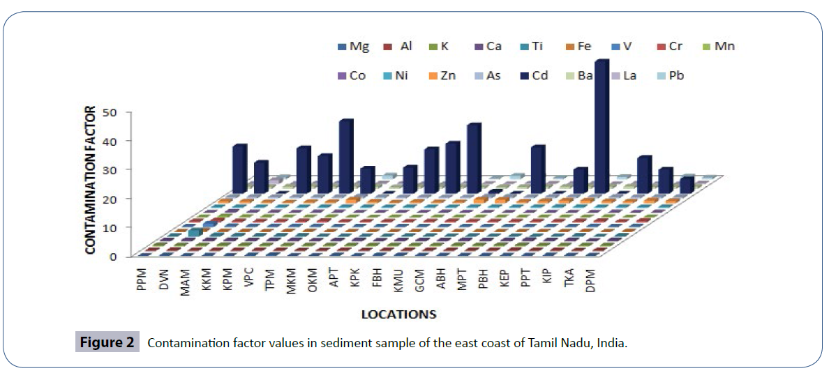
Figure 2 Contamination factor values in sediment sample of the east coast of Tamil Nadu, India.

Pollution load index (PLI)

The pollution load index (PLI) provides a simple, comparative means for assessing the level of heavy metal pollution [23]. PLI is determined as the nth root of the product of nCf

where Cf is the contamination factor and n is the number of metals. According to Tomlinson et al. [23], PLI>1 means that pollution is present; otherwise, if it is below 1, there is no metal pollution. The PLI values are between 0.00 and 0.66, with mean of 0.25. As seen from Table 4, the PLI value of all sediment samples are less than one. This indicates that sediemnts are not polluted by heavy metals. Figure 3 shows the variation of PLI with sampling locations.

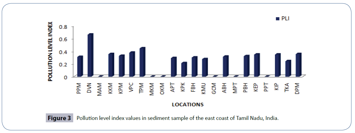
Figure 3 Pollution level index values in sediment sample of the east coast of Tamil Nadu, India.

Potential contamination index (Cp)

The potential contamination index can be calculated by the following method [24].

where (Metal)_{Sample max} is the maximum concentration of a metalin sediment, and (Metal)_Background is the average value of the sediment in a background level. Cp values were interpreted assuggested by Davaulter and Rognerud (2001) [24], where Cp<1 indicates low contamination; 13 is severe contamination. The calculated potential contamination index of heavy metals given in Table 5.

Heavy metals	Cp
Mg	0.281
Al	0.349
K	0.357
Ca	0.566
Ti	2.150
Fe	0.463
V	1.248
Cr	0.688
Mn	0.455
Co	0.374
Ni	0.379
Zn	1.283
As	0.646
Cd	45.66
Ba	0.837
La	1.337
Pb	1.290

Table 5: Potential contamination index (Cp) values of heavy metals in sediment samples of east coast of Tamil Nadu.

The Cp values of heavy metals such as Mg, Al, K, Ca, Fe, Cr, Mn, Co, Ni, As, Ba shows the less than 1 indicates sediemnts are low contaminated by theses metals whereas Cp values of Ti, V, Zn, La and Pb lies between 1 and 3 indicates sediemnts are moderately contaminated by these metals.

But metal Cd shows the greater than 3 shows that sediments are severely contaminated by cdmium. This may be due to influence of anthropogenic activites in the study area. Figure 4 shows the variation of Cp with heavy metals.

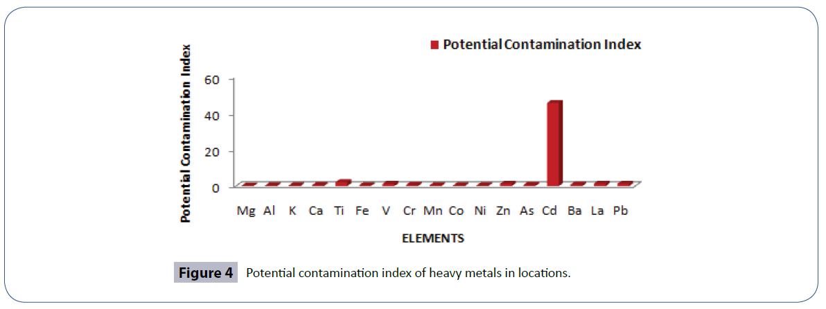
Figure 4 Potential contamination index of heavy metals in locations.

Conclusion

The concnetration of heavy metals has been determined in sediments using EDXRF technique. The low heavy metal content in sediments indicates that sediments not polluted. The CF values show that all sediments are low heavy metal contamination whereas some locations of Thenpattinam (TPM), Koonimedu (KMU), Ganapathichettikulam (GCM) shows that moderate contamination. Also from the potentional contamination index Cp, all sediment samples are low contamination except Ti, V, Zn, La, Pb and Cd. Hence the sediment samples of present study area not much polluted by heavy metals. This work represents the current state of sediment quality from Pattipulam to Dhevanampattinam along the East Coast of Tamilnadu, India that will be a useful tool to authorities in charge of sustainable estuarine and coastal zone management.

Acknowledgement

We are sincerely thanks and gratitude to Dr. K. K. Satpathy, Head, Environment and Safety Division, RSEG, EIRSG, Indira Gandhi Centre for Atomic Research (IGCAR), Kalpakkam- 603 102 for giving permission to make use of EDXRF facility in RSEG and also our deep gratitude and thanks to Dr. MVR Prasad, Head, EnSD, RSEG, IGCAR, Kalpakkam- 603102, India for his keen help and constant encouragements in EDXRF measurements. Our sincere thanks to Mr. KV Kanagasabapathy, Scientific Officer, RSEG, IGCAR for his technical help in EDXRF analysis.

Tables at a glance

References

1. Ives AR, Cardinale B(2004) Foodeweb interactions govern the resistance of communities after non-random extinctions. Nature 429: 174-177.
2. Larison JR, Likens E, Fitzpatrick JW, CrockJG (2000) Cadmium toxicity among wildlife in the Colorado rocky mountains. Nature 406: 181-183.
3. Gao X, Chen CTA (2012) Heavy metal pollution status in surface sediments of the coastal Bohai Bay. Water Research46: 1901-1911.
4. Christophoridis C, Dedepsidis D, Fytianos K (2009) Occurrence and distribution of selected heavy metals in the surface sediments of Thermaikos Gulf, N. Greece. Assessment using pollution indicators. Journal of Hazardous Materials 168: 1082-1091.
5. Larrose A, Coynel A, Schäfer J, Blanc G, Massé L,et al. (2010) Assessing the current state of the Gironde Estuary by mapping priority contaminant distribution and risk potential in surface sediment. Applied Geochemistry 25: 1912-1923.
6. Feng H, Jiang H, GaoW, Weinstein MP, Zhang Q, et al. (2011) Metal contamination in sediments of the western Bohai Bay and adjacent estuaries, China. Journal of Environmental Management 92: 1185-1197.
7. Gao X, Li P(2012) Concentration and fractionation of trace metals in surface sediments of intertidal Bohai Bay, China. Marine Pollution Bulletin 64: 1529-1536.
8. Hu B, Li G, Li J, Bi J, Zhao J, et al. (2013) Spatial distribution and ecotoxicological risk assessment of heavy metals in surface sediments of the southern Bohai Bay, China. Environment Science and Pollution Research 20: 4099-4110.
9. Ravisankar R, Sivakumar S, Chandrasekaran A, Kanagasabapathy KV, Prasad MVR, et al. (2015) Statistical assessment of heavy metal pollution in sediments of east coast of Tamilnadu using Energy Dispersive X-ray Fluorescence Spec troscopy (EDXRF). App RadiaIsot 102: 42-47.
10. Long ER, Field LJ, MacDonald DD(1998) Predicting toxicity in marine sediments with numerical sediment quality guidelines. Environmental Toxicology and Chemistry 17: 714-727.
11. Long ER, Ingersoll CG, MacDonald DD (2006) Calculation and uses of mean sediment quality guideline quotients: a critical review. Environmental Science & Technology 40: 1726-1736.
12. Larsen B, Jensen A(1989) Evaluation of the sensitivity of sediment monitoring stationary in pollution monitoring. Marine Pollution Bulletin 20:556-560.
13. Williams TM, Rees JG, Kairu KK, Yobe AC (1996) Assessment of contamination by metals and selected organic compounds in coastal sediments and waters of Mombasa, Kenya. Technical Report WC.
14. Balls PW, Hull S, Miller BS, Pirie JM, Proctor W(1997) Trace metal in Scottish estuarine and coastal sediments. Marine Pollution Bulletin 34: 42-50.
15. DassenakisM, Scoullos M, Gaitis A(1997) Trace metals transport and behaviour in the Mediterranean estuary of Acheloos river. Marine Pollution Bulletin 34: 103-111.
16. Tam NFY, Wong WS(2000) Spatial variation of metals in surface sediments of Hong Kong mangrove swamps. Environmental Pollution 110: 195-205.
17. Bettinetti R, Giarei C, Provini A (2003) Chemical analysis and sediment toxicity bioassays to assess the contamination of the River Lambro (Northern Italy). Arch Environ ContamToxicol 45: 72-78.
18. Van de Guchte C (1992)The sediment quality triad:an integrated approach to assess contaminated sediments.In: Newman PJ, Piavaux MA, SweetingRA (Eds.), River water quality, ecological assessment and control. Brussels 417-423.
19. Chapman PM(2000) The sediment quality triad: Then, now and tomorrow. International Journal of Environmental Pollution 13: 351-356.
20. Turekian KK, Wedepohl KH(1961) Distribution of the Elements in some major units of the Earth's crust. Geological Society of America, Bulletin 72: 175-192.
21. Herut B, Hornung H, Krom MD, Kress N, Cohen Y (1993)Trace metals in shallow sediments from the Mediterranean coastal region of Israel. Marine Pollution Bulletin 26: 675-682
22. Håkanson L (1980) Ecological risk index for aquatic pollution control: a sediment logical approach. Water Research 14: 975-1001.
23. Tomlinson DC, Wilson JG, Harris CR, Jeffery DW(1980) Problems in the Assessment of Heavy Metals Levels in Estuaries and the Formation of a Pollution Index.HelgoländerWissenschaftlicheMeeresuntersuch 566-575.
24. Davaulter V, Rognerud S(2001) Heavy metal pollution in sediments of the Pasvik River drainage. Chemosphere 42: 9-18.