Keywords: “Reading” of noise\random fluctuations; Trendless sequences.
Differentiation of the sugar solutes taken from different producers; Differentiation of different equipment based on their internal noise.
The frequently used abbreviations:
DW – distilled water
PDF – probability distribution function
TLS – trendless sequence
VAG – voltammogram
Introduction
Now the problem of extraction of information from the measured TLS becomes a central one for researchers associated with creation of new technological processes in chemistry, physicsand engineering. However, part of the researchers tries to extract an information based on some reasonable suppositions. Unfortunately, the principles of the mathematical statistics based on the model suppositions related to the noise does not work properly. Many methods of the mathematical statistics were associated with the straggle/suppression of a noise from the desired trends and they did not concern about the hidden information that are associated with the removed trendless fluctuations.
Only in the end of the last century and in the beginning of our century part of the researchers try to extract some information from random fluctuations defined wrongly as “noise”. In particular, the basics of the fluctuation noise spectroscopy (including also many useful references) is give in the book [1] and papers [2-3]. The applicationof the Mori-Zwanzig formalism was given in the papers [4-5]. Unfortunately, these approaches include some unjustified suppositions and contain some treatment errors. Therefore, in spite of their initial attractiveness, they become useless in analysis of random sequences having different nature. These suppositions and their analysis are listed in paper [6]. The essential results were obtained from analysis of electrochemical noise [7-12], other type of ‘noises’ as understanding of the earthquakes phenomenon and their quantitative description, analysis of medical data is given in papers [3,4,13,14]. Unfortunately, in spite of these promising attempts the general picture associated with analysis of arbitrary types of random sequences (especially TLS) is absent. It is very desirable to develop the “modeless” method that should be free from treatment errors. This method should contain the errors that accompanies any measurement and should be free from some suppositions related to a nature of random fluctuations. Is it possible to propose this “universal” method? From the first glance, it looks like a “crazy” idea. However, two papers [6, 19] published recently by the author allow to hope that this universal tool can be created.
In this paper the author wants to add another universal method associated with analysis of distribution of the amplitudes. Usually, it was accepted to consider that the distribution of the amplitudes of some random trendless sequence is described by the Gaussian distribution function. If the noise is uniform then the sequence of the ranged amplitudes (SRA) coincides with the segment of the straight line. Many researchers in contrast to the Gaussian distribution consider the long-tail distributions as Pareto [15], Levy [16] and other generalized distributions. However, these proposed distributions were not tested properly in the fitting of a wide set of data (it is not a simple procedure, especially for Levy distribution) and the absence of some definite criteria of their application makes their application is questionable. Therefore, any practitioner needs some PDF, which can be suitable for the fitting of a wide set of data because it helps to reduce to a minimal set of the fitting parameters of the chosen data.
The description of the method and proposed algorithm
In this method, one can consider another distribution that is tested on available data and it can be considered as a potential candidate for the fitting of real data. This distribution is described by the following formula
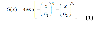
One can notice also that in many cases it is necessary to change the variables x « y in expression (1) and take into account that the roots can be complex-conjugated, i.e. . Besides, this interesting finding that forces to reconsider the conventional understanding of the probability distribution function (PDF), it is necessary to take into account another useful formula that evaluates quantitatively the quality of the performed experiment. Really, let us realize that any experiment can be performed in the form of rectangle matrix (N´M), where j=1,2,…,N; m=1,2,…,M determine the number of data points and number of repeated measurements, correspondingly.
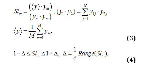
Expression forms a symmetrical matrix with the values located in the interval (0, 2). If the values of this matrix located in the interval (1,2) that the quality of this experiment can be considered as “good”. If some values lie in the interval (0,1) it means that some measurements can be considered as unsatisfactory and should be removed. The essential share of the unsatisfactory measurements forces to admit the experiment as “bad” or as nonstationary, when the influence of uncontrollable factors become essential or predominant. We should take into account the results obtained in papers [17, 18], when the statistical similarity was obtained based on the statistics of the fractional moments and selection of a “good” measurement based on the distribution of the slopes of the corresponding measurement relatively its mean value
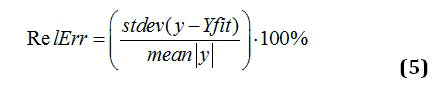
If the most of the values of Slm (m = 1,2,…,M) are located in the interval then this experiment can be acknowledged as “good”. In quantitative evaluations the well-known “3-sigma” criterion was used [17,18].The amplitude distribution function (1) allows to reduce N data points to 7 fitting parameters (5 from Eqn.(1) plus2: RelErr value and the Pearson correlation coefficient). The value of the fitting error is defined by the conventional expression
Simple expressions (1) and (2) are sufficient for solution of the problem formulated above.
The treatment of the available data
Differentiation of the sugar solutes obtained from different producers
From Dr. A. Sidelnikov (Electrochemical laboratory, Ufa Oil University) the author obtained the voltammograms (VAGs) for the microcurrents (10-8A) of the distilled water (DW). These VAGs were obtained in the form of 10 matrices measured during 5 days. Each cycle for the chosen substance occupied 2 hours as the period of measurements includingalso one hour break without removing the measured electrodes. Each rectangle matrix gives N=1190 data points and M=100 successive measurements. In the same manner, the sugar solutes (75g/L)obtained from the sugar sandsand taken from 4 different producers were prepared. These solutes were measured in the same conditions as the distilled water: normal conditions (room temperature (20±1.5)°C, normal pressure (760 ± 20) mm Hgand the controlled humidity – 60%). In order not to create an additional advertisementto the chosen sugar producer we define them as Sg-1,2,3,4, correspondingly. The successive treatment stages are shown in Figs. 1(a,b). In Fig.1(a) we compare two initial VAGs (DW and Sg-1). The values of the current were increased in 104 times and OX axis corresponds to number of data points decreased in N/102 times. Fig.1(b) shows the corresponding integral curves for the same VAGs. As one can see from this figure the differences between two compared VAGs are clearly seen. If we form the corresponding SRAs (Fig.1(b))from these integral curves then one can use them for quantitative comparison with each other. These curves can be fitted with the help of Eqn.(1) and thereby to reduce the initial matrices (N´M) to the matrices (M´7). The fitting curves are shown in Fig.2. In Figs 3(a) we show the distribution of all measurements for the distilled water evaluated by means of expression (2). Figure 3(b) shows the distribution of the maximal/minimal correlations, correspondingly. The same correlations are observed for all sugar solutes; therefore, these figures are not shown. The further analysis shows that the most sensitive and stable parameter in comparison with other fitting parameters is the height of the SRA clearly seen in Fig.1 (b). This observation allows to receive the compact matrix having the size M´Cl.Where Cl=1,2,…,10 parameter corresponds to the 10 heights obtained for all M=100 successive measurements). Similarly, we obtain 4 matrices having the same size for each sugar solute. The final results of their comparison obtained with the help expression (2) are listed in Table 1. As it follows from Table -1 all statistical parameters in this table are located in the interval (0,1). This result solves the problem formulated above- the statistical parameters of the distilled water and mixtures accompanying each sugar solute are statistically different. In similar experiments it is rather difficult to find a distinct parameter that has monotone behavior with respect to monotone changings of some external factor. The expression (1) allows giving this possibility.
The statistical differentiation of two electrochemical devices
Another experiment was related with comparison of random fluctuations recorded from two similar devices (Elins – P-20X and P-40X, Chernogolovka, Russia). The basic problem can be formulated as follows.
Is it possible to notice the statistical differences between these compared devices based on their “internal” fluctuations? As these “internal” fluctuations the background VAGs without electrodes having the currents 10-8A were considered. In order to obtain the distinctive samplings each device was subjected by the constant monitoring during 10 hours. In the result 10 matrices (each recorded matrix has the size [N=2000´M=100]) were obtained. For further analysis each VAG was increased in 108 times and the number of data points was normalized by decreasing in N/103 timesfor treatment convenience. Preliminary comparison of data points taken randomly from two devices show that the SRA(s) formed from the normalized VAGs can serve as the most sensitive parameter that can be used for their differentiation. See Figs. 4 and 5 for details. Again, Eqn. (1) and its fitting parameters can be used for reduction of the initial matrices. Figure 5 demonstrate the fit of the SRAs by the function (1). Figures 6 (a,b,c) demonstrate the distribution of the some fitting parameters over all 100 successive measurements. Analysis of these figures shows that the fitting of the amplitude a figuring in function (1) is preferable and can be chosen as the most stable. Other parameters as it follows from Figs 6(b,c) are not so stable and demonstrate a weak difference between each other. All fitting parameters are not shown because they have similar behavior. Figure 7 shows the “quality” of the performed experiments. As it follows from these figures the values of correlations lie in the interval (1.85, 2) that demonstrates the high correlations of these experiments for the both devices that participate in this comparison.
Results and Discussion
In this paper, we show the possibilities of expression (1) that allows fitting PDF of the amplitudes for a wide class of the TLS. In contrast to other proposed distributions, expression (1) is simple for the fitting purposes and allows finding the most distinct parameter that is used further for differentiation purposes. The comparison vector is listed in Table 2 that undoubtedly demonstrates the difference between specific fluctuations of two similar devices participating in this procedure.
We should notice also the usefulness of expression (2) that can be used for evaluation of stability of measurements that were obtained in any experiment. It cannot use any supposition in contrast to expressions (3) and (4) that were based on “3-sigma” criterion used earlier [17, 18] for evaluation of the strongly-correlated sequences.
The author thinks that these new elements in treatment of TLS(s) will find a wide application in solution of many practical problems.
References
- F. Timashev(2007) Flikker-noise spectroscopy information in Chaotic signals. PhysMatLit publishing house. 248
- F. Timashev,Yu.S. Polyakov(2007) Review of flicker noise spectroscopy in electrochemistry. Fluctuations and Noise Letters. 7: 15-47
- F. Timashev,S. A. Demin,O. Yu. Panischev,Yu. S. Polyakov,A. Ya. Kaplan,Yu. A. Nefedev et al. (2012) Uchenye Zapiski Kazanskogo Universiteta. Seriya Fiziko-Matematicheskie Nauki. 154: 4 161â??177
- M. Yulmetyev(2000) Stochastic dynamics of time correlation in complex systems with
- discrete time 62 6178â??6194
- 5 .R. Yulmetyev(2002) Quantication of heart rate variability by discrete nonstationarity
- non-Markov stochastic processes Phys. Rev. E 65 046-107
- Nigmatullin,R.R.,Vorobev,A.S.,(2019) The universal Set of Quantitative Parameters for
- Reading of the Trendless Sequences. Fluctuation and Noise Letters 18: 4
- A. Tyagai(1977) Faradaic noise of complex electrochemical reactions. ectrochimica Acta. 16 1647 - 1654
- C. Barker Faradaic reaction noise. Journal of Electroanalytical Chemistry and Interfacial Electrochemistry. 82 145-155
- Bozdech, K. Krisher, D.A.Crespo-Yapur, E. Savonova,F. Bonnefont(2016) 1/f2 noise in bistable electro catalytic reactions on mesoscale electrodes. Faraday discussions. 193 187-205
- R. Nigmatullin,S. Martemianov,Yu.K. Evdokimov,E. Denisov,F. Thomas,N. Adiatantov et al. (2016) New approach for PEMFC diagnostics based on quantitative description of quasi-periodic oscillations. International Journal of Hydrogen Energy. 41 12582-12590
- Astafev (2019) Electrochemical noise measurements methodologies of chemical power sources. Instrumentation Science & Technology 47 233-247
- Astafev, A. Uksche (2019) Peculiarities of hardware for electrochemical noise measurement in chemical power sources. IEEE Transactions on Instrumentation and Measurement. 68 4412-4418
- Gutenberg,C.F. Richter Seismicity of the Earth and associated phenomena â?? Princeton. NJ: Princeton University Press. 1949:310
- Nigmatullin, R.R., Vorobev, A.S., Nepeina, K.S., Alexandrov, P.N et al. (2019) Fractal description of the complex beatings: How to describe quantitatively seismic waves? Chaos, Solitons and Fractals 120 171â??182
- E. J. Newman (2005) Power laws, Pareto distributions and Zipf's law. Contemporary Physics. 46:5 323â??51
- Ahsanullah, Valery B. Nevzorov (2014) Some Inferences on the Levy distribution. Journal of Statistical Theory and Applications. 13: 3 205-211
- R. Nigmatullin, Wei Zhang, Renhuan Yang, Yaosheng Lu, Guido Maione et al. (2017) Universal Fitting Function for Quantitative Description of Quasi-Reproducible Measurements. Journal â??Computer Communication & Collaborationâ?ÃÂ. 5:2 2292-1036
- Raoul R. Nigmatullin (2017) The general theory of the Quasi-reproducible experiments: How to describe the measured data of complex systems?â?ÃÂ. Journal â??Communications in Nonlinear Science and Numerical Simulations. 42 324-341