Journal of Heavy Metal Toxicity and Diseases Open Access

Keywords

Sediment; EDXRF; Pollution indices; Potential ecological risk

Introduction

Human activities on land, in the water and air contribute the contamination of seawater and organisms with potentially toxic substances [1,2]. A high level of land use change has led to a strong risk of heavy metal contamination in coastal ecosystems [2-5]. Inappropriate land use has been discussed as a factor that can affect coastal ecosystem health over many years, and clearly, changes in how land is used to directly reflect changing human activities in recent decades [6-11]. Marine pollution is a serious concern in worldwide. Coastal and estuarine regions are considered as the important sinks for the persistent of pollutants. Accumulation of heavy metals occurs in sediment in aquatic environments by biological and geochemical mechanisms and become toxic to sedimentdwelling organisms and fish, resulting in death, reduced growth, or in impaired reproduction and lower species diversity [12]. Sources of metals in aquatic sediments are natural or anthropogenic sources [13,14]. Sediment pollution by heavy metals has been regarded as a critical problem in marine environments because of their toxicity, persistence and bioaccumulation. So it is necessary to investigate the distribution and pollution degree of heavy metal, in order to interpret the mechanism of transportation and accumulation of pollutants and to provide basic information for coast utilization and supervision [15,16].

The present study investigated the assessment of heavy metal pollution in the sediments from Thazhankuda to kodiyakkarrai of the East Coast of Tamilnadu, India. The study area chosen for the heavy metals analysis due to a variety of industrial activities (such as metal smelting, pharmaceuticals etc.) and agriculture activities (which include maize, cassava, sugarcane and vegetables farming) takes place and may enhance the pollution level. These activities may release toxic and potentially hazards to the environment of the study area. So this research is geared up to assess the metal pollution and influence of sources from the toxic metals in the sediments from East Coast of Tamilnadu. The main objective of this work is [1] to determine concentrations of metals present in sediments using EDXRF technique [2] to evaluate the metal contamination of sediments using the pollution indices [3] to identify the sources of heavy metals influenced by of natural and/or anthropogenic [4] to report the findings.

Materials and Methods

Study area

Sediment samples were collected from Thazhankuda to Kodiyakkaraialong the Bay of Bengal coastline during the premonsoon condition. Table 1 lists geographical latitude and longitude of the sampling locations of the study area.

S.No.	Sample ID	Latitude(N)	Longitude(E)	Location
1	CTK	11°46'7.06"	79°48'40.40"	Thazhankuda
2	CDM	11°43'46.84"	79°48'11.39"	Devanampattinum
3	COT	11°43'5.30"	79°48'11.73"	Singarrathoppu
4	CAP	11°35'11.38"	79°47'0.66"	Ayyampet
5	CSP	11°32'56.29"	79°46'48.59"	Samiyarpet
6	CPT	11°31'23.26"	79°47'15.73"	Parangipet
7	CPM	11°24'41.34"	79°50'13.01"	Pichavaram
8	KDM	11°22'53.02"	79°50'28.13"	Kodiyampalayam
9	NPZ	11°19'57.07"	79°51'2.77"	Pazhaiyar
10	NSI	11°13'48.86"	79°52'7.23"	Sirkazhi
11	NPB	11° 8'34.55"	79°52'42.17"	Poombukar
12	TRGB	11° 1'31.97"	79°52'53.12"	Tharangambadi
13	PKK	10°54'59.40"	79°52'12.23"	Karaikal
14	NGR	10°49'16.46"	79°52'21.05"	Nagore
15	NAP	10°44'42.24"	79°52'33.60"	Akkaraipettai
16	VLK	10°41'2.93"	79°52'35.61"	Velankanni
17	TPI	10°37'39.79"	79°52'49.71"	Thirupoondi
18	VKT	10°33'16.64"	79°53'15.85"	Vettaikaranthoppu
19	VED	10°22'58.20"	79°55'37.80"	Vedaranium
20	KODI	10°19'55.85"	79°58'1.53"	Kodiyakkarai

Table 1: The geographical latitude and longitude for the sampling locations at the study area.

Recent industry developments during the last two decades in Cuddalore, Karaikal and Nagapattinam coastal towns include offshore oil production, chemical, fertilizer processing plants and more than 150 small scale industries, all located in this region makes attention for sediment analysis. The recent development of a minor harbor in Nagapattinam town is very important because it acts as the main fishing harbor with heavy movement of fishing and naval vessels in this region. The study area is also drained by the tributaries of river Cauvery which runs through many industrial towns and its tributaries, i.e. rivers Puravandayanar, Vettar, Uppanar pass through the agricultural belt of Tamilnadu state and finally drain into the Bay of Bengal in this coastal sector [17].

Sample collection and preparation

Sediment samples were collected by a Peterson grab sample from a distance of 10 m inside the sea (parallel to the shoreline) along the 20 locations during May 2012. These samples were collected pre-monsoon season, when sediment texture and ecological conditions can be clearly observed, when erosional activities are predominant, and sediments were not transported from the river and estuary towards the beach and marine [18]. Figure 1 shows the location map of the study area. Peterson grab sampler is ideal for near shore sampling with sea bottom having sand, silt or gravel type of sediments. This is the universal method of sediment sample collection for sea bottom sediment sampling at near shore environment [19-21]. Uniform quantity of sediment samples were collected from all the sampling locations. Around 25 cm thick sub-surface samples from the sea bed were collected by the grab sampler. The top sediment layer was scooped with an acid washed plastic spatula. From this 10 cm thick sediment layer was sampled from the middle of the grab. The collected samples were immediately transferred to polythene bags and refrigerated at -4°C until analysis.

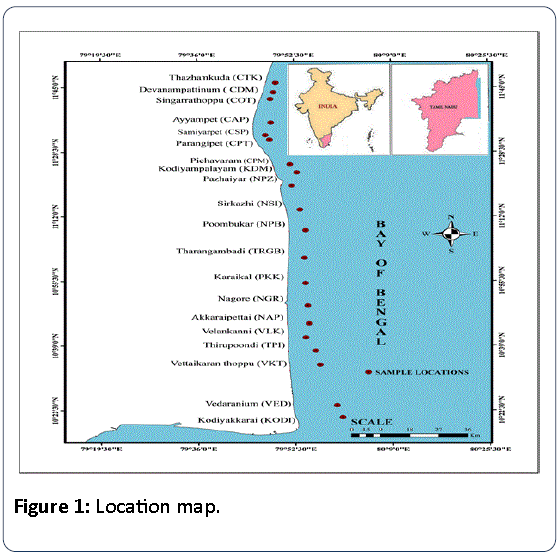
Figure 1: Location map.

The samples were dried at 105°C for 2 h to a constant weight and sieved using a 63 μm sieve in order to identify the geochemical concentrations [22-24]. The grain size of <63 μm, presents several advantages: (1) heavy metals are mainly linked to silt and clay; [2] this grain size is like that of the suspended matter in water; and [3] it has been used in many studies on heavy metal contamination. The samples were then ground to a fine powder using an agate mortar. All powder samples were stored in a desiccator until they were analyzed. One gram of the fine ground sample and 0.5 g of boric acid (H₃BO₃) were mixed. The mixture was thoroughly grinded and pressed into a pellet of 25 mm diameter using a hydraulic press (20 tons) [25].

EDXRF technique

The prepared pellets were analysed using the EDXRF available at Environmental and Safety Division, Indira Gandhi Centre for Atomic Research (IGCAR), Kalpakkam, Tamilnadu. The instrument used for this study consists of an EDXRF spectrometer of model EX-6600SDD supplied by Xenemetrix, Israel. The spectrometer is fitted with a side window X-ray tube (370 W) that has Rhodium as anode. The power specifications of the tube are 3-60 kV; 10-5833 μA. Selection of filters, tube voltage, sample position and current are fully customizable. The detector SDD 25 mm2 has an energy resolution of 136 eV ± 5 eV at 5.9 keV Mn X-ray and 10 sample turret enables keeping and analysing 10 samples at a time. The quantitative analysis is carried out by the In-built software nEXT. A standard soil (NIST SRM 2709_a) was used as reference material for standardizing the instrument. This soil standard obtained from a follow field in the central California San Joaquin valley. The soil standard (reference material) (NIST SRM 2709_a) analysis value are given in Table 2 which reports the certified values with measured EDXRF and its shows that they are well agreement with each other.

Element	Certified Values	EDXRF values
Mg	14600	14900 ± 1000
Al	72100	68400 ±2300
K	20500	19100 ± 700
Ca	19100	16500 ± 500
Ti	3400	3100 ± 100
Fe	33600	33900 ±1200
V	110	98.8 ± 6.59
Cr	130	112.1 ± 4.01
Mn	529	568.2 ± 19.85
Co	12.8	12.8 ± 0.55
Ni	83	69.3 ± 2.98
Zn	107	127.9 ± 4.88

Table 2: Analysis of soil standard-NIST SRM 2709aby EDXRF (mgkg^-1).

Assessment of sediment contamination

Sediments have the capability to record the history and indicate the degree of pollution. To assess the degree of pollution for giving heavy metal requires that the pollutant metal concentration to be compared with an unpolluted reference material (geochemical background). Absence of background values of metal concentrations in Indian estuarine systems made us to use the reference material. The reference material represents a benchmark to which the metal concentrations in the polluted samples are compared and measured. Many authors have used the average shale values or the average crustal abundance data as reference baselines.

In this work average shale values are used for reference material for background values.

Contamination factor (CF)

The level of metal contamination can be expressed by the contamination factor (CF). CF is the ratio between the metal content in the sediment to the background value of the metal [26]. It is an effective tool for monitoring the pollution over a period of time and it is calculated as follows

According to Hakanson [27] CF<1 indicates low contamination; 16 is very high contamination.

Pollution load index (PLI)

The Pollution load index (PLI) represents the number of times by which the heavy metal concentrations in the sediment exceeded the background concentration, and give a summative indication of the overall level of heavy metal toxicity in a particular sample and is determined as the nth root of the product of nCF.

PLI=(CF₁×CF₂×CF₃×........×CF_n)^1/n (2)

Where CF_n is the CF value of metal n. It gives simple and comparative means for assessing the heavy metal pollution level in the sediment sample. The PLI values are interpreted into two levels as polluted (PLI>1) and unpolluted (PLI<1) [25-29].

Contamination degree (C_d)

To facilitate pollution control, Hakanson [27] proposed a diagnostic tool named as ‘degree of contamination’. C_d and it is determined as the sum of the CF for each sample:

The C_d is aimed at providing a measure of the degree of overall contamination in surface layers in a particular core or sampling site. Hakanson [27] proposed the classification of the degree of contamination (mC_d) in sediments as:

C_d<6 Low degree of contamination

6d<12 Moderate degree of contamination

12d<24 Considerable degree of contamination

C_d> 24 High degree of contamination

Modified degree of contamination (mC_d)

The modified degree of contamination was introduced to estimate the overall degree of contamination at a given site according to the formula [30]:

Where n-number of analyzed elements and i=ith element (or pollutant) and CF-contamination factor. The modified formula is generalized by defining the degree of contamination (mC_d) as the sum of all the contamination factors (CF) for a given set of sediment pollutants divided by the number of analyzed pollutants. Using this generalized formula to calculate the mC_d allows the incorporation of as many metals as the study may analyses with no upper limit. The expanded range of possible pollutants can thus include both heavy metals and organic pollutants should later be available for the studied samples.

For the classification and description of the modified degree of contamination (mC_d) in the sediment, the following gradations are proposed: mC_d<1.5 is nil to a very low degree of contamination; 1.5 ≤ mC_d< 2 is a low degree of contamination; 2 ≤ mC_d<4 is a moderate degree of contamination; 4 ≤ mC_d<8 is a high degree of contamination; 8 ≤ mC_d<16 is a very high degree of contamination; 16 ≤ mC_d<32 is an extremely high degree of contamination; mC_d ≤ 32 is an ultra-high degree of contamination.

Potential contamination index (C_p)

The potential contamination index can be calculated by the following method.

Where (Metal) sample Max is the maximum concentration of a metal in sediment, and (Metal) Background is the average value of the same metal in a background level. C_p values were interpreted as suggested by Dauvalter and Rognerud [31,32] where C_p<1 indicates low contamination; 1p<3 is moderate contamination; and C_p>3 is severe contamination.

Assessment of potential ecological risk

Hakanson [27], proposed a method for the potential ecological risk index (RI) to assess the characteristics and environmental behavior of heavy metal contaminants in sediments. The main function of this index is to indicate the contaminant agents and where contamination studies should be prioritized. The potential ecological risk index (RI) is calculated as the sum of all risk factors for heavy metals in sediments, is the monomial potential ecological risk factor, CF is the contamination factor, and is the toxic response factor, representing the potential hazard of heavy metal contamination by indicating the toxicity of particular heavy metals and the environmental sensitivity to contamination. According to the standardized toxic response factor proposed by Hakanson Cr, As, Ni, Pb and Zn have toxic response factors of 2, 5, 5, 5 and 1 respectively. The formula of the potential ecological risk index is given below

The terminology used to describe the risk factors and RI was suggested by Hakanson [27], where: <40 indicates a low potential ecological risk; 40<<80 is a moderate ecological risk; 80< <160 is a considerable ecological risk; 160<<320 is a high ecological risk and > 320 is a very high ecological risk. RI<95 indicates a low potential ecological risk; 95 380 is a very high ecological risk.

Results and Discussions

Table 3 summarizes the determined heavy metal concentration of the study area by using energy dispersive Xray fluorescence (EDXRF) technique. The concentration of the heavy metal varies from 800-10100 mg/kg^-1 for Mg; 38600-70600 mg/kg^-1 for Al;12100-16100 mg/kg^-1 for K; 8900-29100 mg/kg^-1 for Ca; 1000-21200 mg/kg^-1 for Ti; 7900-47100 mg/kg^-1 for Fe; 30.1-314.6 mg/kg^-1 for V; 38.1-312.6 mg/kg^-1 for Cr; 159.8-1171.3 mg/kg^-1 for Mn; 2.8-16.6 mg/kg^-1 for Co; 23.9-44 mg/kg^-1 for Ni and 26-87.3 mg/kg^-1 for Zn. The most abundant metal in the sediments among the heavy metals is found to be Aluminum (Al) [25]. The mean order of metal concentration is Al>Fe>Ca>K>Mg>Ti>Mn>Cr>V>Zn>Ni>Co in the study area.

S.No.	Sample ID	Mg	Al	K	Ca	Ti	Fe	V	Cr	Mn	Co	Ni	Zn
1	CTK	8800	66100	15600	29100	5100	22100	80.2	86.4	477.9	7.9	30.8	48.8
2	CDM	4100	48200	14100	14100	2100	9600	35.3	38.5	187.2	3.5	24.2	26.8
3	COT	3200	47900	13300	14700	2600	10600	44.6	45.6	216.1	3.8	23.9	28.1
4	CAP	4400	52100	13600	14300	3200	14800	48.3	77.5	297.8	5.5	31.5	34.4
5	CSP	4600	54000	14100	15400	2700	14100	45.5	66.2	271.4	5.2	29.5	36.4
6	CPT	6100	60000	13900	18300	3900	19700	64.8	101.8	425	7.1	37.4	47.3
7	CPM	9500	56700	13400	17300	13800	37200	223.9	232.9	745.1	12.8	41.6	69.7
8	KDM	1700	42900	15500	9900	1100	8600	31.1	38.1	180.9	2.9	29.1	26.4
9	NPZ	800	38600	13900	8900	1000	7900	30.1	38.9	159.8	2.8	27.6	26
10	NSI	4900	48100	14900	13100	2200	12500	40.7	63.6	257.1	4.6	26.9	32.8
11	NPB	2400	43500	15000	12000	1800	11300	35.4	61.2	232.3	4	25.9	29.8
12	TRGB	7900	61300	15400	21000	15400	38200	238.6	271.8	811.3	13	42.7	65.6
13	PKK	7700	70600	14300	24600	21200	47100	314.6	312.6	1171.3	16.6	44	87.3
14	NGR	6200	56800	16100	20200	5100	20000	91.1	141.2	445.1	7	35.6	49.3
15	NAP	8100	58000	15400	18900	5200	20400	77.1	120.1	451.9	7.4	34	44.6
16	VLK	6700	43000	12100	12200	1900	10600	39.8	62.5	232.4	4	25.8	32.9
17	TPI	9300	59700	13600	20600	10200	29900	155.7	174.7	680	10.5	38.9	64.6
18	VKT	7900	58300	14100	20000	2600	16200	52.3	105.2	342.8	5.9	33	39.1
19	VED	10100	57500	13000	20900	5700	22500	102.5	142.9	531.3	8.1	34.3	44.7
20	KODI	5300	57900	13100	20300	4200	18800	77	121.9	433.3	6.7	32.8	38.1
Average		5985	54060	14220	17290	5550	19605	91.4	115.2	427.5	7.0	32.5	43.6
Max Value		10100	70600	16100	29100	21200	47100	314.6	312.6	1171.3	16.6	44	87.3
Bac Value		15000	88000	26600	16000	4600	47200	130	90	850	19	50	95
Cp		0.673	0.802	0.605	1.819	4.609	0.998	2.420	3.473	1.378	0.874	0.880	0.919

Table 3: Heavy metal concentration (mg kg^-1) in sediments along the East Coast of Tamilnadu, India.

The locations of Karaikkal(PKK), Tharangambadi (TRGB), Pichavaram (C_pM)are characterized by higher concentrations of Al, Ti, Fe, V, Cr, Mn, Co and Zn when compared with other locations. This may be due to the high tourists’ boat activities and other anthropogenic activities like shipping and harbor activities, industrial and urban wastage discharges, dredging, etc.

The calculated CF values are given in Table 4.

S.No.	Sample ID	Mg	K	Ca	Ti	Fe	V	Cr	Mn	Co	Ni	Zn	PLI
1	CTK	0.59	0.59	1.82	1.11	0.47	0.62	0.96	0.56	0.42	0.45	0.51	0.68
2	CDM	0.27	0.53	0.88	0.46	0.20	0.27	0.43	0.22	0.18	0.36	0.28	0.34
3	COT	0.21	0.50	0.92	0.57	0.22	0.34	0.51	0.25	0.20	0.35	0.30	0.37
4	CAP	0.29	0.51	0.89	0.70	0.31	0.37	0.86	0.35	0.29	0.46	0.36	0.46
5	CSP	0.31	0.53	0.96	0.59	0.30	0.35	0.74	0.32	0.27	0.43	0.38	0.45
6	CPT	0.41	0.52	1.14	0.85	0.42	0.50	1.13	0.50	0.37	0.55	0.50	0.60
7	CPM	0.63	0.50	1.08	3.00	0.79	1.72	2.59	0.88	0.67	0.61	0.73	1.00
8	KDM	0.11	0.58	0.62	0.24	0.18	0.24	0.42	0.21	0.15	0.43	0.28	0.28
9	NPZ	0.05	0.52	0.56	0.22	0.17	0.23	0.43	0.19	0.15	0.41	0.27	0.24
10	NSI	0.33	0.56	0.82	0.48	0.26	0.31	0.71	0.30	0.24	0.40	0.35	0.41
11	NPB	0.16	0.56	0.75	0.39	0.24	0.27	0.68	0.27	0.21	0.38	0.31	0.35
12	TRGB	0.53	0.58	1.31	3.35	0.81	1.84	3.02	0.95	0.68	0.63	0.69	1.05
13	PKK	0.51	0.54	1.54	4.61	1.00	2.42	3.47	1.38	0.87	0.65	0.92	1.25
14	NGR	0.41	0.61	1.26	1.11	0.42	0.70	1.57	0.52	0.37	0.52	0.52	0.67
15	NAP	0.54	0.58	1.18	1.13	0.43	0.59	1.33	0.53	0.39	0.50	0.47	0.65
16	VLK	0.45	0.45	0.76	0.41	0.22	0.31	0.69	0.27	0.21	0.38	0.35	0.39
17	TPI	0.62	0.51	1.29	2.22	0.63	1.20	1.94	0.80	0.55	0.57	0.68	0.90
18	VKT	0.53	0.53	1.25	0.57	0.34	0.40	1.17	0.40	0.31	0.49	0.41	0.54
19	VED	0.67	0.49	1.31	1.24	0.48	0.79	1.59	0.63	0.43	0.50	0.47	0.72
20	KODI	0.35	0.49	1.27	0.91	0.40	0.59	1.35	0.51	0.35	0.48	0.40	0.59
Average		0.40	0.53	1.08	1.21	0.42	0.70	1.28	0.50	0.37	0.48	0.46	0.59
Cd		7.98	10.69	21.61	24.13	8.31	14.07	25.60	10.06	7.33	12.99	9.19
mcd		0.66	0.89	1.80	2.01	0.69	1.17	2.13	0.84	0.61	1.08	0.77

Table 4: Contamination factor (CF), Pollution load index (PLI), Contamination Degree (Cd) and Modified Degree of Contamination (mCd) of sediments along the East Coast of Tamilnadu, India.

From the CF values, considerable contaminations were noticed in the locations like Tharangambadi (TRGB) and Karaikal (PKK) with the values of 3.35 and 4.61 for Ti; 3.02 and 3.47 for Cr respectively, and also moderate contamination was observed with 1.31 and 1.54 values for CA; 1.84 and 2.42 for the Vin Tharangambadi (TRGB) and Karaikal (PKK) respectively. The locations of Pichavaram (C_pM), Tharangambadi (TRGB) and Karaikal (PKK) was not contaminated by Mg, K, Fe, Mn, Co, Ni and Zn. Figure 2 shows the variation of contamination factor with location.

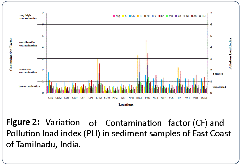
Figure 2: Variati o n of Contamin a ti o n factor (CF) and Pollution load index (PLI) in sediment samples of East Coast of Tamilnadu, India.

As seen from Table 4, pollution load index (PLI) ranged from 0.24-1.25, with mean value 0.59. PLI value of all sediment samples is less than one except locations of Pichavaram (C_pM), Tharangambadi (TRGB) and Karaikal (PKK). This indicates that the sediments are not polluted by heavy metals. The moderately polluted locations of Pichavaram (C_pM), Tharangambadi (TRGB) and Karaikal (PKK) in this study may be due to the anthropogenic activities. Figure 2 shows the variation of PLI values with different locations.

Table 4 lists the contamination degree (C_d) of sediment samples of the east coast of Tamilnadu, India. The C_d values of 7.98 for Mg; 10.69 for K; 21.61 for Ca; 24.13 for Ti; 8.31 for Fe; 14.07 for V; 25.60 for Cr; 10.06 for Mn; 7.33 for Co; 12.99 for Ni; 9.19 for Zn. Moderate degree of contamination was observed in Co, Mg, Fe, Zn, Mn and Fe; Ni, V and Ca shows the considerable degree of contamination; Ti and Cr shows high degree of contamination from its value. This may be due to the recent increase in major industrial (in the coastal areas) and a minor harbor activity that involves movement of naval vessels throughout the year may increase the contamination levels in coastal areas. Figure 3 shows the variation of C_d values of heavy metals in locations.

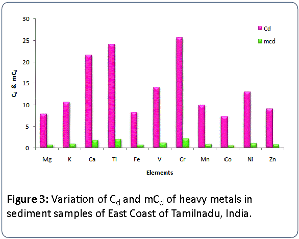
Figure 3: Variation of C_d and mC_d of heavy metals in sediment samples of East Coast of Tamilnadu, India.

The mC_d values are between 0.6 and 2.1 for the studied elements. Cr and Ti showed mC_d values >2 indicating a moderate degree of contamination (Table 4). From the analysis of mC_d values indicating that Nil to moderate degree of contamination in study area. Figure 3 shows the variation of mC_d values of heavy metals in locations.

Table 3 reports the potential contamination index (C_p) of sediment samples. The C_p values of heavy metals except Ti shows less than one indicates that the sediments are low contamination. A severe contamination was observed for Ti (4.609) in the sediments may be due to influence of anthropogenic activities in the study area. Figure 4 shows the variation of C_p values of heavy metals in locations.

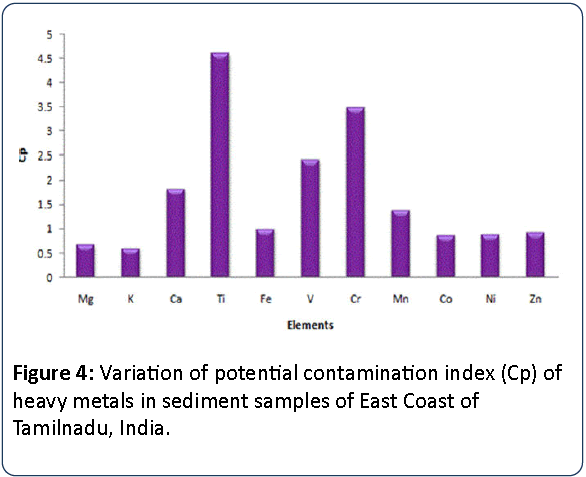
Figure 4: Variation of potential contamination index (Cp) of heavy metals in sediment samples of East Coast of Tamilnadu, India.

As seen from the Table 5, the values of Cr, Ni and Zn found to be less than 40 indicates that the sediments are low potential ecological risk. But potential ecological risk index of Cr, Ni and Zn were less than 95 indicates that low potential ecological risk index (RI). Hence sediments of the present study area showed low potential ecological risk.

Conclusion

Distribution and ecological risk for Mg, Al, K, Ca, Ti, Fe, V, Cr, Mn, Co, Ni and Zn in sediment samples were studied. From the analysis, the sediments are not polluted by Mg, Al, K, Ca, Ti, Fe, V, Mn, Co but slightly enriched with Cr, Ni and Zn due to anthropogenic activities. The locations of Pichavaram (C_pM), Tharangambadi (TRGB) and Karaikal (PKK) were found to be moderately polluted by heavy metals due to anthropogenic activities. Heavy metals of Ti and Cr are noticed moderately polluted in the sediments of the study area may be due to human activities.

The value of C_d shows a high degree of contamination for Ti and Cr due to the recent increase in major industries and a minor harbor activity in the coastal areas. The overall range of mC_d values indicates a Nil to moderate degree of contamination in the study area. The values of C_p for all heavy metals show low contamination whereas Ti shows severe contamination due to the influence of anthropogenic activities in the study area. The result shows that there is no potential ecological risk in the study area. The present work indicated that continuous monitoring and efforts of remediation are may be required to improve the coastal environment near industrialized areas.

Acknowledgement

We are sincerely thanks and gratitude to Dr. K. K. Satapathy, Head, Environment and Safety Division, RSEG, EIRSG, Indira Gandhi Centre for Atomic Research (IGCAR), Kalpakkam-603 102 for giving permission to make use of EDXRF facility in RSEG and also our deep gratitude and thanks to Dr. M. V. R. Prasad, Head, EnSD, RSEG, IGCAR, Kalpakkam-603102, India for his keen help and constant encouragements in EDXRF measurements. Our sincere thanks to Mr. K.V. Kanagasabapathy, Scientific Officer, RSEG, IGCAR for his technical help in EDXRF analysis.

References

1. Die´zS, Lacorte S, Viana P, Barcelo D, Bayona JM (2005) Survey of organotin compounds in rivers and coastal environments in Portugal 1999-2000, Environ Poll 136: 525- 536.
2. Maanan M(2008) Heavy metal concentrations in marine molluscs from the Moroccan coastal region, Environ. Poll 153: 176-183.
3. Acevedo-Figueroa D, Jiménez BD, Rodriguez-Sierra CJ(2006) Trace metals in sediments of two estuarine lagoons from Puerto Rico, Environ. Pollut 141: 336-342.
4. Maanan M(2007) Biomonitoring of heavy metals using Mytilusgalloprovincialis in Safi coastal waters, Morocco, Environ. Toxicol 22: 525-531.
5. Flower RJ, Appleby PG, Thompson JR, Ahmed MH, Ramdani M, et al. (2009) Sediment distribution and accumulation in lagoons of the southern Mediterranean region (the MELMARINA Project) with special reference to environmental change and aquatic ecosystems, Hydrobiologia 622: 85-112.
6. BaptistaNeto JA, Smith BJ, McAllister JJ (1999) Sedimentological evidence of human impact on a nearshore environment: Jurujuba Sound, Rio de Janeiro State, Brazil, Appl. Geogr 19: 153-177.
7. Bellucci LG, Frignani M, Paolucci D, Ravanelli M (2002) Distribution of heavy metals in sediments of the Venice lagoon: the role of the industrial area, Sci. Total. Environ 295: 35-49.
8. Patz JA, Daszak P, Tabor GM, Aguirre AA, Pearl M, et al. (2004) Unhealthy landscapes: policy recommendations on land use change and infectious disease emergence, Environ. Health Perspect 112: 1092-1098.
9. PielkeRA (2005) Land use and climate change, Science 310: 1625-1626.
10. Accornero A, Gnerre R, Manfra L (2008) Sediment concentrations of trace metals in the Berre lagoon (France): an assessment of contamination,Arch. Environ. Contam.Toxicol 54: 372-385.
11. Fang SB, Xu C, Jia XB, Wang BZ, An SQ(2010) Using heavy metals to detect the human disturbances spatial scale on Chinese Yellow Sea coasts with an integrated analysis J. Hazard. Mater 184: 375– 385.
12. Szefer P, Glassby GP, Pempkowiak J, Kaliszan R (1995) Extraction studies of heavy-metal pollutants in surficial sediments from the southern Baltic Sea off Poland, Chem. Geol 120: 111-126.
13. Singh KP, Mohan D, Singh VK, Malik A (2005) Studies on distribution and fractionation of heavy metals in Gomti river sediments- a tributary of the Ganges, India, J. Hydrol 312: 14-27.
14. Khaled A, El Nemr A, El Sikaily A (2006) An assessment of heavy-metal contamination in surface sediments of the Suez Gulf using geoaccumulation indexes and statistical analysis, Chem. Ecol 22: 239-252.
15. Long ER, Field LJ, MaC_donald DD(1998) Predicting toxicity in marine sediments with numerical sediment quality guidelines, Environ. Toxico Chem 17: 714-727.
16. Long ER, Ingersoll CG, MaC_donald DD (2006) Calculation and uses of mean sediment quality guideline quotients: a critical review, Environ Sci Tech 40: 1726-1736.
17. Stephen-Pichaimani V, Jonathan MP, Srinivasalu S, Rajeshwara-Rao N, Mohan SP (2008) Enrichment of trace metals in surface sediments from the northern part of Point Calimere, SE coast of India, Environ Geol 55:1811-1819.
18. Ravisankar R, ChandramohanJ,Chandrasekaran A, Prince PrakashJebakumar J, Vijayalakshmi I, et al. (2015) Assessments of radioactivity concentration of natural radionuclides and radiological hazard indices in sediment samples from the East coast of Tamilnadu, India with statistical approach, Mar Pollut Bull 97:419-430.
19. Chatterjee M, Silva Filho EV, Sarkar SK, Sella SM, Bhattacharya A, et al. (2007) Distribution and possible source of trace elements in the sediment cores of a tropical macrotidal estuary and their ecotoxicological significance Environ. Int 33:346-356. 
20. Ingham A (Ed.) (1975) Sea Surveying, New York: John Wiley andSons, pp:306.
21. Sly PG (1969) Bottom sediment sampling, in Proceedings of the 12th Conference on Great Lakes Research, Buffalo, N.Y. International Association for Great Lakes Research, 883-898.
22. Bryan GW, Langston WJ (1992) Bioavailability, accumulation and effects of heavy metals in sediments with special reference to United Kingdom estuaries: a review, Environ Pollut 76:89-131.
23. Buchanan JB (1984) Sediment analysis In: Holme NA, McIntyre AD(Eds). Methods for thestudy of marine benthos, Blackwell Scientific Publications, London41-65.
24. Langston WJ, Spence SK (1994) Metal analysis In: Calow P (Ed.) Handbook of Ecotoxicology. Oxford Blackwell Sci. Publ. London 45-78.
25. Ravisankar R, Sivakumar S, Chandrasekaran A, Kanagasabapathy KV, Prasad MVR, et al. (2015) Statistical assessment of heavy metal pollution in sediments of east coast of Tamilnadu using Energy Dispersive X-ray Fluorescence Spectroscopy (EDXRF), App Radia Isot 102: 42-47.
26. Turekian KK, WedepohlKH (1961) Distribution of the elements in some major units of the Earth’s crust, Geol Soc Am Bull 72: 175-192.
27. Hakanson L (1980) An ecological risk index for aquatic pollution control: a sedimentological approach, Water Res 14: 975-100 1.
28. Tomlinson DL, Wilson JG, Harris CR, Jeffrey DW(1980) Problems in the assessment of heavy-metal levels in estuaries and the formation of a pollution index, Helgoland, Mar. Res 33: 566-575.
29. Harikumar PS, Nasir UP, MujeebuRahman MP(2009) Distribution of heavy metals in the core sediments of a tropical wetland system, Int J Environ Sci Technol 6: 225-232.
30. Abrahim GMS, Parker RJ (2008) Assessment of heavy metal enrichment factors and the degree of contamination in marine sediments from Tamaki Estuary, Auckland, New Zealand, Environ. Monit. Assess 136: 227-238.
31. Dauvalter V, RognerudS (2001) Heavy metal pollution in sediments of the Pasvik River drainage, Chemosphere 42: 9-18.
32. Chandramohan J, Chandrasekaran A, Senthilkumar G, Elango G, Ravisankar R (2016) Heavy Metal Assessment in Sediment Samples Collected From Pattipulam to Dhevanampattinam along the East Coast of Tamilnadu Using EDXRF Technique, J Heavy Metal ToxiDisea 1:1-9.